How to Interpret SPSS Output for One Way ANOVA (October 2026)

A one-way ANOVA in SPSS produces four output tables, and you read them in a fixed order: Descriptive Statistics, Test of Homogeneity of Variances, the ANOVA table, and Post Hoc Tests. Each table answers a different question, and the answer to one decides what you do with the next. Knowing how to interpret SPSS output for one way ANOVA means working through those tables in sequence rather than scrolling straight to Sig. and copying a number.

This guide follows the standard interpretation practice described in APA style guidance, using a worked example with three study methods and 90 students throughout. Menu labels are the ones in IBM SPSS Statistics 26 to 29, and the output layout has been stable since the PASW era. Last reviewed October 2026.

Table of Contents

1. 1The SPSS One-Way ANOVA Output at a Glance
2. 2What You Need
3. 3The Output Tables You Need to Find
4. 4The Design Details That Change the Interpretation
5. 5The Version and Menu Path
6. 6The Assumptions You Must Have Checked
7. 7Step-by-Step: How to Interpret SPSS Output for One Way ANOVA
8. 8Check That You Ran the Correct One-Way ANOVA
9. 9Read the Descriptive Statistics Table First
10. 10How to Interpret the ANOVA Table in SPSS
11. 11Check the Effect Size and the Confidence Intervals
12. 12Interpret the Post Hoc Tests Table
13. 13Check Homogeneity of Variances and the Other Assumptions
14. 14Report the One-Way ANOVA in APA Style
15. 15The Two SPSS Dialogs and Why Your Output Looks Different
16. 16Common Interpretation Mistakes
17. 17Frequently Asked Questions
18. 18What does Sig. mean in SPSS one-way ANOVA?
19. 19Is an ANOVA result significant when Sig. is less than 0.05?
20. 20Why do I need post hoc tests after a significant ANOVA?
21. 21What should I do if Levene’s test is significant in SPSS?
22. 22Is a one-way ANOVA appropriate when there are only two groups?
23. 23Can I report only the ANOVA p-value?
24. 24Conclusion: Start With the ANOVA Table

The SPSS One-Way ANOVA Output at a Glance

Before you read a single number, know which table you are looking at. In the Output Viewer, tables appear stacked in the order SPSS produced them, and the tree on the left lets you jump between them by name.

Output table	What it tells you	What you do with it
Descriptive Statistics	Group means, standard deviations, N and 95% confidence intervals	Read first so you know the pattern before seeing the inferential test
Test of Homogeneity of Variances (Levene’s)	Whether group variances can be treated as equal	If Sig. is below .05, switch to the Welch output and Games-Howell
ANOVA	F statistic, degrees of freedom and Sig. for the overall test	Decide whether the group means differ at all
Post Hoc Tests	Which specific pairs differ, with adjusted significance	Report each significant pair, not the whole table
Effect size (Partial Eta Squared)	How much variance group membership explains	Judge practical importance, not just statistical significance

What You Need

Four things need to be in front of you before interpretation starts: the output tables, the design behind them, the assumption checks, and the version of SPSS that produced them. Here is what each one gives you.

The Output Tables You Need to Find

Open the Output Viewer window and look at the title SPSS generated for your analysis, usually the dependent variable followed by the word ANOVA. Scroll from there. You are looking for the tables listed in the at-a-glance table above, and nothing else is relevant to this interpretation.

If your Output Viewer contains two or more ANOVA analyses, each one gets its own title block and its own set of tables. Scroll to the title that names your dependent variable and your factor. That is the block you interpret, and the other block belongs to a different analysis.

The Design Details That Change the Interpretation

Three pieces of information control whether the output can be interpreted as planned. First, the number of groups: a one-way ANOVA needs three or more levels in the factor, because with two groups you use an independent-samples t-test. Second, the measurement level of the factor, which needs to be nominal or ordinal. Third, the dependent variable, which needs to be continuous, and any covariates you entered.

If you entered covariates, the output contains a Tests of Between-Subjects Effects table instead of the plain ANOVA table, and the row for your factor is the one you report.

The Version and Menu Path

Two menu paths produce a one-way ANOVA: Analyze > Compare Means > One-Way ANOVA, and Analyze > General Linear Model > Univariate. Both are correct, and they produce different output. Report whichever path you actually used, because your supervisor may ask which one.

The Assumptions You Must Have Checked

Levene’s test appears inside the ANOVA output, so you have that one already. Normality does not, and SPSS has no automatic normality check inside the one-way dialog. Run Analyze > Descriptive Statistics > Explore, move your dependent variable into the Dependent List, click Plots, tick Normality plots with tests, and read the Shapiro-Wilk row for each group.

Independence of observations is a design question rather than a number. Each participant should appear in one group only, and one person’s score should not shape another’s. Random assignment handles this best.

Step-by-Step: How to Interpret SPSS Output for One Way ANOVA

Work through the seven steps below in order. Each one produces a decision that the next step depends on, so skipping ahead to the Sig. column is what produces the interpretation errors listed later in this guide.

Check That You Ran the Correct One-Way ANOVA

Confirm three things in the dialog you used, not in the output. The factor box must hold a variable with three or more groups, the dependent list must hold a numeric score variable, and the model box must be set to one factor. If you also ticked Welch’s test or effect size in the Options dialog, an extra row or an extra column appears in the output, and both are explained below.

Check the group labels too. Unlabelled values of 1, 2 and 3 produce a table that is statistically fine and impossible to report, because nothing tells you which group is which. Go back to the variable view and add value labels before you interpret anything.

Read the Descriptive Statistics Table First

Here is the human-readable version of your results: the actual score for each group, how much those scores varied, and how confident you can be about each mean. Read it before the ANOVA because it tells you the direction and rough size of any effect, which makes the inferential tables easier to interpret.

Five columns matter, and each tells you something different. N is the number of valid scores in that group, and the three N values should add up to your total sample. Mean is the group average. Std. Deviation is how spread out the individual scores are within that group. Std. Error is the standard deviation divided by the square root of N, which is the typical distance of a single score from the group mean. The 95% Confidence Interval gives the range within which the population mean most likely sits.

Standard deviation is about individual variation. Standard error is about the precision of the mean. They are different quantities and students swap them constantly, so check which one you are quoting.

Group	N	Mean	Std. Deviation	Std. Error	95% CI
Flashcards	30	72.43	8.20	1.50	69.37 to 75.49
Videos	30	78.93	9.10	1.66	75.53 to 82.33
Group work	30	74.15	7.80	1.42	71.59 to 76.81

Read the confidence intervals before you look at anything inferential. Overlapping intervals are a warning, not a verdict. Here the videos interval sits above the other two, which matches the mean pattern, and the flashcards and group work intervals overlap heavily.

How to Interpret the ANOVA Table in SPSS

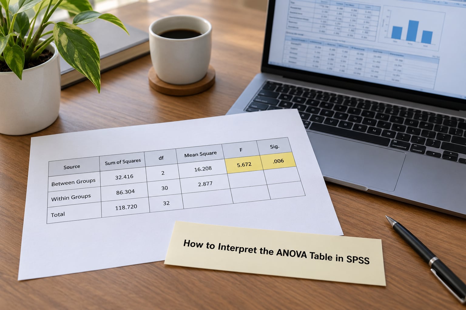
This is the table everybody opens, and it is the one most people read badly. Three rows appear: Between Groups, Within Groups and Total. The Between Groups row measures how much your group means differ from the overall mean. The Within Groups row measures the ordinary scatter of scores inside each group. The Total row is the sum of the two, and it represents all the variation in your dependent variable.

Each column is one calculation step, and SPSS prints them all because each feeds the next.

Column	Plain English meaning	In the worked example
SS (Sum of Squares)	Total variation in scores, split into between-group and within-group parts	Between 680.6, Within 6115.8, Total 6796.4
df (Degrees of Freedom)	Number of independent pieces of information, estimated by the data	2, 87, 89
MS (Mean Square)	Sum of squares divided by degrees of freedom	340.3, 70.3, 76.4
F	Between-groups mean square divided by within-groups mean square	340.3 / 70.3 = 4.84
Sig.	The p-value attached to that F, compared against your alpha level	.010

The F statistic is a ratio, and this is the single most misunderstood number in the output. If the null hypothesis were true, group membership would explain nothing, and the between-groups mean square would be no larger than the within-groups mean square by chance alone. So F sits near 1 when the null holds. An F of 4.84 means the variation between groups is nearly five times the variation inside groups, which is unusual under the null.

The degrees of freedom follow a simple rule worth learning once. The total df equals N minus 1, because one number is spent estimating the overall mean: 90 minus 1 equals 89. The between-groups df equals the number of groups minus 1: three minus 1 equals 2. The within-groups df is what is left over, 89 minus 2 equals 87. That is why the df in your table add up to the total, and a table where they do not add up means something has gone wrong with the run.

The Sig. column is a p-value, and it answers one question: if the group means were genuinely equal in the population, how likely would you be to see differences at least this large? Here Sig. equals .010, so a ten-in-one chance. Because .010 is below the conventional alpha level of .05, the result is statistically significant and the null hypothesis of equal population means is rejected.

The alpha level of .05 is a convention, not a law. Some fields use .01, and if you set your alpha before seeing the data, that is the threshold you apply afterwards.

Note what the sums of squares are not. They are not your result. Students quote SS values in write-ups because they sit at the top of the table and look important, but they carry no standalone meaning. APA reporting wants the F statistic, its degrees of freedom, the p-value and an effect size.

Check the Effect Size and the Confidence Intervals

A significant p-value tells you a difference is unlikely to be chance. It says nothing about whether the difference matters, and a large sample makes small p-values easy to produce. This is where effect size earns its place in your results paragraph.

To see it, open the Options dialog back in the One-Way ANOVA dialog and tick Effect size, then re-run. Partial Eta Squared appears as an extra column on the right of the ANOVA table. It represents the proportion of variance in the dependent variable that group membership explains, ranging from 0 to 1. In the worked example it is .100, meaning group membership accounts for about ten per cent of the variation in exam scores.

Conventional benchmarks, following Cohen, put partial eta squared below .01 as a small effect, around .06 as medium and .14 or above as large. These are rough reference points from another design, not thresholds your data must clear.

The descriptive confidence intervals give you a second read on practical importance. Two group means separated by a fraction of a standard deviation rarely matter in practice, no matter how small the p-value is.

Interpret the Post Hoc Tests Table

A significant ANOVA tells you only that at least one group mean differs from another. It never tells you which pair. That is the job of the post hoc table, and SPSS produces it only if you ticked a post hoc test in the Post Hoc dialog before running the analysis.

Tukey is the default choice for one-way ANOVA when variances are equal, and it controls the familywise error rate across all pairwise comparisons, so the chance of any false positive across the whole set stays at your alpha level. Bonferroni is more conservative and useful when you planned a small number of specific comparisons in advance. Dunnett compares every group against one named control group. Games-Howell is the option when variances are unequal.

Comparison (I – J)	Mean Difference	Std. Error	Sig.	Adjusted Sig.
Videos – Flashcards	6.50	2.16	.003	.008
Videos – Group work	4.78	2.16	.029	.061
Flashcards – Group work	-1.72	2.16	.430	.690

Read the Adjusted Sig. column, not the Sig. column. Sig. is the raw p-value for that single pair before any correction, and it always looks more impressive. Adjusted Sig. has the familywise error control applied, so only pairs at or below .05 count as significant. Here that leaves one finding: videos scored higher than flashcards by 6.50 points. The videos and group work comparison looks close to significant at .029 raw, and adjusting for three comparisons moves it to .061, which is not significant.

The sign of Mean Difference shows direction. A positive value means group I scored higher than group J. A negative value means the reverse.

Below the pairwise table you will find Homogeneous Subsets, which SPSS prints as columns of letters. Groups that share at least one letter are not significantly different from each other. Groups with no letter in common differ. In this analysis the letters read videos as a, flashcards as b and group work as b, which encodes exactly one significant pair and is the same result the adjusted Sig. column gave you.

A mean plot confirms the pattern visually. Tick Plot means in the Options dialog and SPSS draws the group means with 95% confidence interval error bars. Non-overlapping bars correspond to a significant difference in most cases, which makes this a quick sanity check before you write anything up.

Check Homogeneity of Variances and the Other Assumptions

Levene’s test sits in its own small table between Descriptives and ANOVA. The Sig. value is the p-value for the null that all group variances are equal. If it is above .05, the homogeneity assumption is not violated and the standard ANOVA output stands. If it is below .05, variances differ and the standard F test cannot be trusted.

In this analysis Levene’s test gives F equal to 0.41 with Sig. equal to .663, comfortably above .05, so the standard output is the one to report. Group standard deviations of 8.20, 9.10 and 7.80 support that reading.

When Levene’s test is significant, tick Welch’s test in the Options dialog and re-run. SPSS adds a Welch’s Test row to the ANOVA table with its own F, degrees of freedom and Sig., and a second Robust Tests table gives the adjusted comparisons. Use the Welch’s row for your F and p-value, and choose Games-Howell as the post hoc test. If Welch’s Sig. comes back non-significant, your conclusion changes, so read it rather than assuming the standard row still applies.

For normality, read the Shapiro-Wilk Sig. for each group in the Explore output. Above .05 means no evidence against normality, which is the normal result for group sizes above about 30. Below .05 does not destroy the analysis for large samples, because the one-way ANOVA is reasonably tolerant of moderate departures; with small groups, transform the variable or fall back on a non-parametric alternative.

For independence, check the design rather than the output. If one participant contributed several scores, the observations are not independent and the p-values are too small.

Report the One-Way ANOVA in APA Style

APA reporting for a one-way ANOVA names the test, the F statistic, its degrees of freedom, the p-value and an effect size, preceded by the descriptive statistics. Two templates cover most results.

For a significant result: A one-way ANOVA was conducted to compare exam scores across three study methods. The videos group (M = 78.93, SD = 9.10) scored significantly higher than the flashcards group (M = 72.43, SD = 8.20), F(2, 87) = 4.84, p = .010, partial eta squared = .100. Tukey post hoc comparisons showed no other significant differences.

For a non-significant result, the wording changes and students get this wrong most often. Write F(2, 87) = 1.12, p = .327, partial eta squared = .025, and then say that the analysis did not find a statistically significant difference between the group means. Do not write that the null was proven, that the groups are the same, or that the hypothesis was confirmed.

Degrees of freedom are always written as F(2, 87), the between-groups value first. Omit the leading zero on p values and effect sizes, so p equals .010 rather than p equals 0.010, and keep the decimals to two or three places.

The Two SPSS Dialogs and Why Your Output Looks Different

Students who search for an interpretation guide often find output that does not match the tables described in tutorials. The reason is almost always which dialog produced it, and both are legitimate.

Dialog	Output tables produced	When to use it
Analyze > Compare Means > One-Way ANOVA	Descriptives, Levene’s, ANOVA, Post Hoc, Homogeneous Subsets	One factor, no covariates. The usual choice for a simple comparison
Analyze > General Linear Model > Univariate	Descriptives, Levene’s, Tests of Between-Subjects Effects, Post Hoc, Model Summary, residual plots	Covariates, multiple factors, or partial eta squared by default

The GLM Univariate route puts everything in the Tests of Between-Subjects Effects table, with the F, Sig. and Partial Eta Squared columns on one row per factor. Read your factor’s row the same way as the ANOVA table. If you ran both dialogs on the same data, SPSS produced two separate blocks of output, and the two are equivalent for a single factor with no covariates.

Levene’s is present in both layouts, which means you can always check variance homogeneity without leaving the output you already have.

Common Interpretation Mistakes

Every one of these produces a defensible-looking sentence that a marker or supervisor will spot. The fix is usually a change of wording rather than a change of analysis.

Writing that Sig. is the probability the null hypothesis is true. It is not. Sig. .010 means that, if the population means were equal, you would see differences this large in about one run out of a hundred. It is the probability of the data you observed under the null, not the probability of the null itself.

Saying you rejected the alternative hypothesis. You either reject the null or you fail to reject it. Nobody rejects the alternative hypothesis, and writing that you did it signals that the p-value was misread.

Reporting the sum of squares as the finding. Between Groups SS of 680.6 means nothing on its own. Report F, its degrees of freedom, p and an effect size instead.

Quoting Sig. from the post hoc table instead of Adjusted Sig. The raw Sig. ignores the multiple comparisons problem. Only Adjusted Sig. carries the correction.

Claiming every pair differs because the ANOVA was significant. A significant F guarantees at least one differing pair, never all of them. Here one of three pairs survived adjustment, and writing that all three groups differed would overstate the finding.

Reading Levene’s Sig. backwards. A significant Levene’s test means variances are unequal, which invalidates the standard F test. Reporting the standard row anyway is the most damaging error on this list.

Overstating a non-significant result as proof of no difference. Failing to reject the null means the data did not provide enough evidence to reject it. Small, real differences are easy to miss with small samples.

Ignoring descriptive statistics entirely. Reporting that groups differ without a single group mean leaves a reader unable to understand the pattern.

Citing a menu path you did not use. If your methods section says Compare Means and your output came from Univariate, expect the question. State the path you actually followed.

Frequently Asked Questions

Conclusion: Start With the ANOVA Table

Open the output on the ANOVA table first. Read Sig. against your chosen alpha level, and that single number tells you whether you need a post hoc section at all. If it is not significant, report F, df and p and stop there, because no pairwise comparison is warranted.

If it is significant, add the effect size, then read the Adjusted Sig. column of the post hoc table and report only the pairs that survived correction. Write the sentence your evidence supports, using the descriptive means to describe rather than the sums of squares, and remember that a one-way ANOVA shows a difference between group means without explaining why that difference exists.