How to Run an Independent Samples t Test in SPSS (2026)

To run an independent samples t test in SPSS, go to Analyze > Compare Means > Independent-Samples T Test, move your numeric outcome variable into the Test Variable(s) box, move your two-group categorical variable into the Grouping Variable box, define the group codes, and click OK. The whole procedure takes about two minutes once your data is coded correctly.

• Analyze > Compare Means > Independent-Samples T Test opens the dialog box.
• Put the continuous score in Test Variable(s) and the two-group variable in Grouping Variable.
• Click Define Groups, enter the two codes SPSS found for your groups, click OK, then click OK again.

The rest of this guide walks through what to check before you start, how to read the two output tables without guessing, and how to write the result up so a marker can see the numbers you based it on.

Table of Contents

1. 1What You Need
2. 2Step-by-Step
3. 3Step 1: Check and Prepare Your Data
4. 4Step 2: Check Whether the Groups Are Independent
5. 5Step 3: Run the Test in SPSS
6. 6Step 4: Interpret the SPSS Output
7. 7Step 5: Report the Result
8. 8Common Mistakes
9. 9Frequently Asked Questions
10. 10What does an independent samples t test in SPSS compare?
11. 11How do I interpret Levene’s test in SPSS?
12. 12Why is my independent samples t test not significant?
13. 13Should I use the equal variances assumed or equal variances not assumed row?
14. 14How do I report an independent samples t test in APA format?
15. 15What should I do if my data are skewed or contain extreme outliers?
16. 16Conclusion

What You Need

An independent samples t test compares the mean of one continuous variable between two separate, unrelated groups. You need one numeric dependent variable, one categorical grouping variable that splits your cases into exactly two groups, and enough cases in each group for the means to be worth comparing.

Typical examples: a satisfaction score for a treatment group against a control group, mean salary for respondents grouped by gender, or exam marks for undergraduates against postgraduates. What ties them together is that no participant appears in both groups.

Before you open the dialog box, get these four things straight:

• Your dependent variable must be numeric and measured at interval or ratio level. A score, a duration, a count, a salary in pounds all qualify.
• Your grouping variable must have exactly two values. If it has three or more, you want a one-way ANOVA instead.
• Know the group codes. Open Variable View and read the numbers under the Values column for your grouping variable, because Define Groups needs the codes, not the labels.
• Know your SPSS version. In SPSS Statistics 27 and 28 the menu reads Compare Means and Proportions; in 29 and later it reads Compare Means. Everything after that menu is identical.

The test rests on four assumptions, and SPSS only checks one of them for you.

1. Continuous dependent variable. Scores measured on a scale, not categories.
2. Two independent groups. Different people in each group, or at least separate observations with no pairing.
3. No extreme outliers in either group. A single wild value can drag a mean and inflate the standard deviation.
4. Approximate normality within each group. With small samples under about 30 per group this matters most.

Homogeneity of variance, the assumption that both groups spread out by a similar amount, is the fifth one, and SPSS does test it for you through Levene’s test. You do not have to guess whether to trust it; the output tells you.

If you are not sure which test fits your design, this table settles it quickly.

Your design	Test to use in SPSS	Menu path
Two unrelated groups, one numeric outcome	Independent samples t test	Analyze > Compare Means > Independent-Samples T Test
The same people measured twice, such as pre and post scores	Paired samples t test	Analyze > Compare Means > Paired-Samples T Test
Three or more unrelated groups	One-way ANOVA	Analyze > Compare Means > One-Way ANOVA
Two unrelated groups but an ordinal outcome, or a badly skewed score	Mann-Whitney U test	Analyze > Nonparametric > Independent Samples

Getting this wrong is the single most common error students make, and it is easier to make than it looks. A test of a treatment group against a control group where each participant only received one condition is independent. A pre and post questionnaire completed by the same 40 people is paired, and using the independent test there throws away the pairing and often changes the answer.

Step-by-Step

Step 1: Check and Prepare Your Data

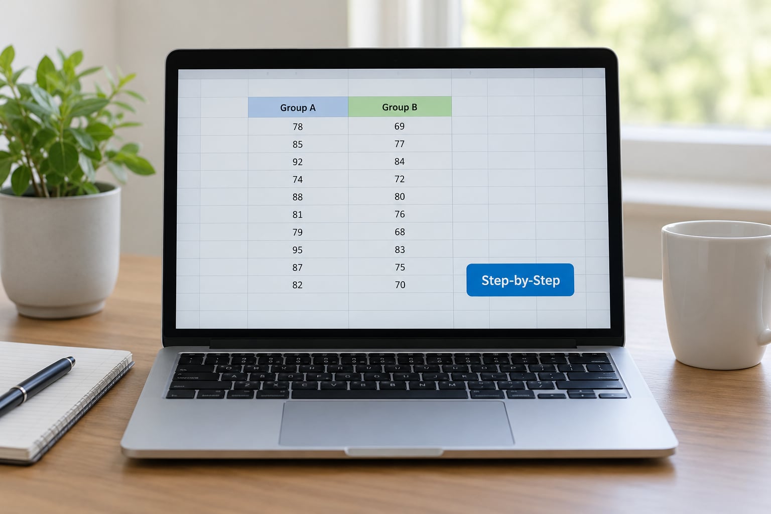
Start in Data View and check the two columns before you analyse anything. Scroll down past the last real case and look for a row of dashes or the value -99, which some researchers use to mark missing data. Those rows will silently shrink your group sizes unless you tell SPSS they are missing.

Right-click any column heading and choose Variable View to confirm the coding. In the Values column, your grouping variable should show two entries such as 1 = Control and 2 = Treatment, or 0 = No and 1 = Yes. Those left-hand numbers are the group codes, and they are exactly what you type into Define Groups later.

If the coding column is empty, SPSS will not let you define groups. Right-click the variable in Variable View, click the cell in the Values column, click Add, type the number on the left of the box and the label on the right, then repeat for the second group.

Step 2: Check Whether the Groups Are Independent

Independence means no case is linked to a case in the other group. If the same participant contributes a score to both groups, the design is paired and the independent test is the wrong choice, no matter how tidy the data looks.

A quick way to sanity check: ask yourself whether you could remove one participant without removing their partner. If the answer is yes, you are fine. If removing someone also removes someone else, you need the paired samples procedure.

Group sizes do not need to be equal. An independent t test handles a 12-person group against a 40-person group without trouble, and the output will show you both N values so you can check nothing was dropped.

Step 3: Run the Test in SPSS

Click Analyze > Compare Means > Independent-Samples T Test. In SPSS 27 and 28 the middle level reads Compare Means and Proportions.

The dialog box opens with a list of available variables on the left and two empty boxes on the right. Click your outcome variable and then the arrow next to Test Variable(s) so it lands in the top box.

Click your grouping variable and use the arrow next to Grouping Variable to move it into the lower box. SPSS does not care about the order of these two, but the grouping variable must be in its own box or nothing will run.

Click Define Groups. A small box opens listing every group code SPSS found in that variable, for example 1 and 2. Type the lower code into Group 1 and the higher code into Group 2, click OK, then click OK on the main dialog.

Tick Options only if you want descriptive statistics. The Statistics default already gives you means, standard deviations, the Levene test, the t statistic, degrees of freedom and the two-tailed significance, which is everything a report needs.

If you would rather run it from syntax, paste this into a new syntax window, replace the variable names with your own, and run it:

T-TEST GROUPS=group(1 2)
/VARIABLES=score
/CRITERIA=CI(.95).

Syntax is worth learning once you are automating analyses, because the result is identical and the command can be saved and re-run without clicking through four dialog boxes every time.

Step 4: Interpret the SPSS Output

The Output Viewer gives you two tables. Read the first one for the descriptive picture and the second one for the decision, and never quote a number from the wrong row.

The Group Statistics table has one column per group. Here is what each column tells you.

Column	What it means
N	How many valid cases landed in that group. Compare it with your expected size to spot dropped cases.
Mean	The average score for that group. The gap between the two means is the effect you are testing.
Std. Deviation	How spread out the scores are within the group.
Std. Error Mean	The standard deviation divided by the square root of N, which is the precision of that mean.

The Independent Samples Test table is where the decision lives. Two rows appear, Equal Variances Assumed and Equal Variances Not Assumed, and the choice between them comes from Levene’s test in the top block.

The rule is short: look at the Sig. column in the Levene’s Test for Equality of Variances row.

• If that Sig. is greater than .05, read the top row, Equal Variances Assumed.
• If it is less than .05, read the bottom row, Equal Variances Not Assumed.

That second row is often called Welch’s t test. It adjusts the degrees of freedom using Satterthwaite’s approximation, which is why the df there is usually a decimal.

On the row you have chosen, read these values:

• t, the t statistic. Its size is how far the mean difference sits from zero in standard error units.
• df, the degrees of freedom, based on the two sample sizes.
• Sig. (2-tailed), the p value. If it is below .05 you reject the null hypothesis and call the difference statistically significant. If it is above .05 you do not have enough evidence to say the groups differ.
• Mean Difference, the direction and size of the gap between the means.
• Std. Error Difference, the precision of that difference.
• 95% Confidence Interval of the Difference, the range you expect the true difference to fall in most of the time. If it contains zero, the result is not significant, which is a useful consistency check.

Here is a worked example using illustrative numbers. Suppose the Group Statistics table shows a treatment mean of 7.42 with a standard deviation of 1.08 on 30 cases, and a control mean of 6.15 with a standard deviation of 1.31 on 30 cases.

Levene’s Sig. comes back at .412, which is above .05, so you read the Equal Variances Assumed row. The output on that row shows t(58) = 4.12, Sig. (2-tailed) = .000, a mean difference of 1.27, and a 95% confidence interval of the difference running from 0.68 to 1.86.

Because Sig. (2-tailed) is below .05 and the confidence interval excludes zero, the treatment group scored significantly higher than the control group. The direction matches the mean difference of 1.27, which is the check most students forget to do.

A significant p value says the difference is unlikely to be sampling noise. It says nothing about whether the difference is big enough to matter in practice, which is why reporting an effect size has become standard. Cohen’s d is the standard measure, and you can get it from the output with the formula d = t × √(1/n₁ + 1/n₂). Plugging the worked example values into d = 4.12 × √(1/30 + 1/30) gives roughly 1.06, a large effect.

Step 5: Report the Result

Report the test with the four numbers that let someone else judge it: the group means, the t statistic, the degrees of freedom, the p value, and an effect size. Round the p value to three decimal places, the t and df to two, and the means to two.

Use this template and fill in your values:

An independent samples t test showed that participants in the treatment group (M = 7.42, SD = 1.08) scored significantly higher than those in the control group (M = 6.15, SD = 1.31), t(58) = 4.12, p < .001, d = 1.06. Levene’s test was not significant (p = .412), so the Equal Variances Assumed row was used.

Change the wording if the difference goes the other way. If the control group scored higher, write that the control group scored significantly higher, and keep the sign of the mean difference and the t statistic negative as SPSS reports them.

For a dissertation results table, a small table with the group means, standard deviations, t, df, p and d is clearer than a paragraph, and it lets a reader see the raw numbers behind the claim.

A bar chart with error bars showing the two group means plus their confidence intervals is a good companion visual. Readers take in the size of the gap faster than they take in a t statistic.

Common Mistakes

Almost every avoidable problem comes from one of four sources: the wrong test, the wrong coding, a skipped assumption check, or a misread output row.

• Using the paired samples test on independent data. Fix: use Independent-Samples T Test whenever different people fill each group.
• Using the paired samples test on genuinely paired data. Fix: if the same participants were measured twice, use Analyze > Compare Means > Paired-Samples T Test and put both measurements in the same pair.
• Coding the groups as text. Fix: a grouping variable made of words like yes and no cannot be used until you assign numeric codes in Variable View.
• Typing the group labels into Define Groups instead of the codes. Fix: enter 1 and 2, not Control and Treatment. SPSS is looking for values, not labels.
• Ignoring Levene’s test and quoting the top row every time. Fix: read the Sig. value, then pick the row it tells you to use.
• Reading Sig. (2-tailed) as a one-tailed probability. Fix: it already covers both tails, so compare it to .05 as it stands.
• Claiming non-significance means the groups are identical. Fix: write that you found no statistically significant difference, then report the effect size and confidence interval to show how much evidence you actually had.
• Reporting a p value only. Fix: add Cohen’s d, because with a large enough sample a trivial difference can reach significance.

Two SPSS error messages account for most of the rest.

Message or symptom	Cause	Fix
The system cannot begin the dialog box for this procedure	No variable of the right type is selected	Click a numeric variable before opening the menu
Group codes are required, or no group codes are defined	You clicked Define Groups and left a box empty, or the grouping variable has no Value labels	Type both codes, and add Values in Variable View if they are missing
The grouping variable is a string variable	Groups were typed as words	Recode the variable to numeric 1 and 2 in Transform > Recode into Different Variables
N in the output is smaller than expected	Missing values coded as -99 or 9	Use Data > Define Missing Values and mark the missing value code
Sig. (2-tailed) is blank	One group has fewer than two cases	Check the N column in Group Statistics and fix the coding or the data

If Levene’s test comes back significant and you do not want to argue about it, run Analyze > Nonparametric > Independent Samples and choose Mann-Whitney U instead. That test does not assume equal variances or normality, which makes it the safe fallback whenever the t test assumptions look shaky.

To check those assumptions directly, open Analyze > Descriptive Statistics > Explore, move the score in and the grouping variable to the Factor box, and click Plots to add a boxplot with means. Outliers show up as dots outside the whiskers, and the Normality table with Kolmogorov-Smirnov and Shapiro-Wilk statistics tells you whether each group departs badly from a normal shape.

Frequently Asked Questions

Conclusion

Start by confirming the two-group structure: one numeric outcome, one categorical variable coded as 1 and 2, and no participant appearing in both groups. Everything after that is four clicks in the Analyze menu.

Then read the output properly. Check the N values so you know nothing was dropped, use Levene’s test to pick between Equal Variances Assumed and Equal Variances Not Assumed, and compare Sig. (2-tailed) with .05 before you claim anything.

Report the group means, t, df, p and an effect size in one sentence. If the assumptions do not hold, say which one failed and switch to Mann-Whitney U rather than hoping the result survives.