How to Run Ordinal Logistic Regression in SPSS, Stata, and R 2026

Ordinal logistic regression predicts an ordered categorical outcome — a 1-to-5 satisfaction rating, a severity band, an exam grade — by modelling the probability of landing in each category or lower. Knowing how to run ordinal logistic regression matters because almost every survey ends up with a Likert-style variable, and the default habits people fall into (treating it as continuous, or defaulting to multinomial) produce numbers they can’t defend. The fit itself takes about twenty minutes once the outcome is coded correctly; the real work is the proportional odds assumption and reading the thresholds properly.

Below is one workflow that runs end to end in all three programs, using the same worked example throughout so you can see that the software differs only at the surface.

Table of Contents

1. 1What You Need — an ordered outcome, coded predictors, and one big assumption
2. 2Step-by-Step — one example, three programs
3. 31. Check whether ordinal logistic regression is appropriate for your data
4. 42. Prepare and inspect the data
5. 53. Run the model in SPSS
6. 64. Run the model in Stata
7. 75. Run the model in R
8. 86. Interpret coefficients, odds ratios, and thresholds
9. 97. Check fit and the proportional odds assumption
10. 108. Save output and prepare the research report
11. 11Common mistakes and the fix for each
12. 12Frequently Asked Questions
13. 13Should I use ordinal logistic regression or multinomial logistic regression?
14. 14Why does my software treat the outcome as continuous instead of ordered?
15. 15What should I do if the proportional odds assumption is violated?
16. 16How do I use an ordinal logistic regression model to predict probabilities?
17. 17Do I need to report the threshold estimates and odds ratios?
18. 18Conclusion — start with the outcome, test the assumption, then read the odds ratios

What You Need — an ordered outcome, coded predictors, and one big assumption

You need a dependent variable whose categories have a genuine, defensible order: strictly disagree through strongly agree, no pain / mild / moderate / severe, fail / pass / merit / distinction. If a respondent could plausibly say that “moderate” sits halfway between “mild” and “severe” in a measurable sense, you have a strong case for the ordinal model rather than a continuous one.

You also need predictors that are already in usable shape. Continuous variables stay numeric; categorical predictors are fine, but you should decide the reference level before you run anything, because the odds ratio you get depends on it. And you need to know which assumption you are making: ordinal logistic regression assumes the proportional odds assumption, meaning that one unit of a predictor shifts the odds of every adjacent category comparison by the same amount on the log-odds scale.

Three things in this list trip people up regularly:

• Ordered categories, not just categories. “Red, green, blue” is nominal. “None, some, all” is ordinal. If the labels have no natural ranking, this is the wrong model.
• Enough cases per category. Sparse categories produce unstable thresholds. As a working rule, keep at least roughly 10 cases in the smallest category, and be especially careful when you have many predictors or small subgroups.
• Enough cases for the model as a whole. There is no dedicated ordinal-logistic module in G*Power, so people borrow a chi-square or small-effect approximation and add a safety margin — or simulate with packages such as simr in R. Rule of thumb: aim for at least 15 to 20 cases per estimated parameter, and treat that as a floor rather than a target.

Know when to walk away. If your outcome has only two categories, use ordinary binary logistic regression — the ordinal model collapses to the same thing but with more explanation to write. If the categories have no order, use multinomial logistic regression. And if you have a genuinely continuous outcome with equal intervals, linear regression is still the right tool.

Step-by-Step — one example, three programs

The running example: satisfaction, a five-point rating from Low to High, explained by age (years), gender (Female, Male, Other), and dose (a treatment level coded 1 to 3). Sample size 600, all complete cases. You will meet the same numbers in all three programs.

1. Check whether ordinal logistic regression is appropriate for your data

Yes if the outcome is ordered categorical with more than two levels, the observations are independent, and the proportional odds assumption is at least defensible. The model is called the proportional odds model, the ordered logit model, or the cumulative logit model — same maths, different software traditions.

It is not the same as linear regression on a 1-to-5 score. Linear regression treats the gap from 1 to 2 as identical to the gap from 4 to 5 and can predict 2.743, which is not a response anyone gave. It is also not multinomial logistic regression: because the model uses one coefficient per predictor instead of one set per outcome category, it needs far fewer parameters, which matters when your sample is moderate and your predictor list is long.

If your response labels are out of order — say, categories are coded 1 = Agree, 2 = Disagree, 3 = Neutral — fix the labels, not the numbers. Recoding so the numbers follow the natural order changes nothing substantive about the data; it just stops the model from sorting your categories wrongly.

2. Prepare and inspect the data

Make the outcome an ordered factor with levels in the correct sequence. This is the single most important preparation step, and skipping it is why people get “continuous” warnings from their software.

Then look at the data before modelling:

• Run frequencies with percentages on the outcome. Note any category with very few cases and any that collapsed entirely.
• Cross-tabulate the outcome by each categorical predictor. If one group sits entirely in one category, that predictor will be hard to estimate.
• Check missing values and decide your handling rule before you fit anything, because listwise deletion will change your effective sample size.
• Check for multicollinearity among continuous predictors. Correlations above .80 between predictors is a reasonable warning sign.
• Confirm independence of rows. If the same people answered twice, or if your data are clustered by school or clinic, you need a mixed model rather than the plain version.

Once you know the counts, you can already anticipate the answer. If satisfaction sits 70 percent in the top two categories for everyone, the model can rank groups but cannot say much about the individual categories — worth stating in your limitations.

3. Run the model in SPSS

In SPSS 29, the path is Analyze > Regression > Ordinal Regression. Put satisfaction in the Dependent box, age in Covariates, and put gender and dose in Factors.

Under Location, choose the category you want as the reference for any categorical factor — SPSS lists them lowest to highest, and the default is the lowest level. Getting this wrong changes your odds ratio without changing the model, which is a common source of confusion. Leave the link function on logit; probit and complementary log-log give you the same predicted probabilities with different coefficient scaling.

The key output is Model Summary, which carries a Test of Proportional Slopes line when you have at least one factor. A non-significant result there means the proportional odds assumption is not contradicted by the data.

The command behind the dialog is PLUM, which you can paste into a syntax window:

PLUM satisfaction BY gender dose WITH age
  /LOCATION gender(1) dose(1)
  /MODEL TYPE=A
  /PRINT=FIT SUMMARY
  /MISSING=LISTWISE
  /TEST=TYPE=PROB.

Note that SPSS’s ordinal dialog is limited compared with the other two. It gives you no confidence intervals for thresholds and no random effects. For those, people usually export to R or Stata.

4. Run the model in Stata

Stata 18 wants an ordered numeric variable. encode creates it from a string, and the labels carry through to the output.

encode satisfaction, gen(sat_o)

ologit sat_o c.age i.gender i.dose, baseoutcome(1)

estat gof
margins, predictpr
margins age, predictpr atmeans
estat vce(cluster id_school)

ologit is the workhorse and is fast on large samples. estat gof gives a goodness-of-fit table comparing observed and predicted frequencies per category, which is the quickest sanity check there is — if observed and predicted line up closely in every row, the model is doing its job. margins, predictpr gives you predicted category probabilities directly, and adding estat vce(cluster id_school) gives standard errors that account for clustering when your rows are not independent.

Stata’s built-in ologit has no Brant test. To test proportional odds, either run the user-written Brant command:

ssc install brant
brant sat_o c.age i.gender i.dose, nrep(500) r(9989)

or fit the generalised ordered model directly with gologit2 from SSC, which fits the proportional odds model first and then relaxes it selectively:

ssc install gologit2
gologit2 sat_o c.age i.gender i.dose, base(1) nolog

The reported p-values in gologit2 tell you which predictors break proportionality.

5. Run the model in R

R 4.3 or later with the ordinal package gives you the most control of the three, and the same package handles mixed models when you need them.

install.packages(c("ordinal", "ggeffects"))
library(ordinal)

df$satisfaction <- factor(df$satisfaction,
                          levels = c("Low", "Low-Medium", "Medium",
                                     "Medium-High", "High"),
                          ordered = TRUE)

m <- clm(satisfaction ~ age + gender + dose, data = df)
summary(m)

The summary() output gives you two blocks: threshold coefficients for the four cut points, and the slope coefficients for age, gender and dose. Exponentiate the slopes for odds ratios with confidence intervals:

ci <- confint(m)
data.frame(
  predictor = names(coef(m)),
  OR  = exp(coef(m)),
  lower = exp(ci[, 1]),
  upper = exp(ci[, 2])
)

For predicted probabilities across a range of a continuous predictor, ggeffects does the work cleanly:

library(ggeffects)
ggeffect("age", model = m, type = "prob")
plot(ggeffect("age", model = m, type = "prob"))

If you have repeated measures on the same people or observations nested in schools, swap clm() for clmm() and add a random intercept:

mm <- clmm(satisfaction ~ age + dose + (1 | id_school), data = df)

MASS::polr() is also worth knowing. It fits the same model faster and gives you thresholds directly, but it has no built-in assumption test and no random effects, which is why most people end up with clm().

6. Interpret coefficients, odds ratios, and thresholds

Each slope coefficient is a log odds ratio for a one-unit increase in that predictor, holding the others constant. Exponentiate it and you get the common odds ratio: the factor by which the odds of being at or above any given category change per unit of the predictor. The same number applies to every adjacent category comparison, and that single shared number is the proportional odds assumption in practice.

Suppose dose returns an odds ratio of 0.33. Moving up one dose level multiplies the odds of being in a higher satisfaction category by 0.33 — a 67 percent reduction in those odds. It is an odds statement, not a probability statement, and it says nothing about which category gains the most. That gap is exactly what predicted probabilities fill.

The thresholds (also called cut points or alpha parameters) work differently. For a five-category outcome there are four of them, and each one is the point on the linear predictor where the cumulative probability crosses a boundary. For a person with a linear predictor of 0.4 and thresholds at -1.2, -0.3, 0.8 and 2.1, the cumulative probabilities are:

Category split	Cut point minus linear predictor	Cumulative probability
P(Low or below)	-1.6	0.17
P(Low-Medium or below)	-0.7	0.33
P(Medium or below)	0.4	0.60
P(Medium-High or below)	1.7	0.85

Exact-category probabilities are the differences between consecutive rows: 0.17, 0.16, 0.27, 0.25 and 0.15. Note what the model does not produce — there is no ordinary intercept and no linear-regression slope here, so do not report the cut points as “the effect of the predictor”.

Statistical significance tells you whether the odds ratio is unlikely to be 1. A wide confidence interval running from 0.2 to 5.5 means you cannot rule out no effect at all, whatever the p value says in a marginal sample.

These values are illustrative, but the conversion from odds to probability is fixed and worth keeping to hand:

Probability	Odds	Log odds (logit)
0.10	0.11	-2.20
0.20	0.25	-1.39
0.50	1.00	0.00
0.80	4.00	1.39
0.90	9.00	2.20

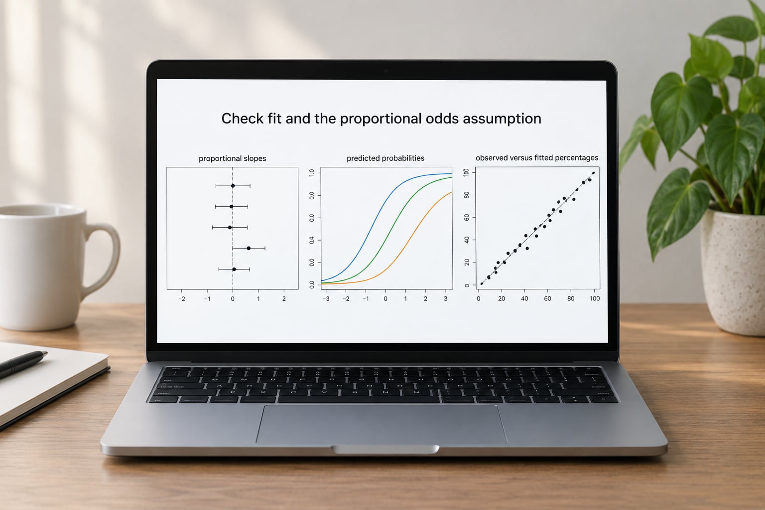
7. Check fit and the proportional odds assumption

Test the proportional odds assumption before you interpret anything. In SPSS, read the Test of Proportional Slopes line in Model Summary. In Stata, run brant or fit gologit2 and read which predictors show non-significant p-values. In R, use the score test from the same package:

nominal_test(m)

A non-significant result is good news — it means the data do not contradict proportional odds. It does not prove the assumption is true; these tests are usually underpowered, particularly with small samples or few predictors, so a non-significant result is permission to proceed rather than a guarantee. Report the test and its p-value either way.

Then run the fit checks:

• Goodness of fit. In Stata, estat gof compares observed and predicted counts per category. In R, compare predicted probabilities against the raw distribution.
• Outliers and influential cases. Look at cases with large residuals or high leverage. Ordinal models are sensitive to a handful of extreme responses on thin categories.
• Sparse cells. Any category with very few cases makes both thresholds and predicted probabilities unstable. Combine categories only if you can justify the combination substantively, not to make a p value appear.
• Calibration. Group cases by predicted probability and compare with observed proportions — a quick predicted-versus-observed plot does more here than a formal test.
• Model comparison. Compare nested models with a likelihood ratio test and AIC; lower AIC is better, and the difference matters more than the absolute value.

If a predictor violates proportional odds, do not quietly delete it. In R, fit a threshold-varying model and test the change:

m2 <- clm(satisfaction ~ age + gender + dose,
         threshold = ~ age, data = df)
anova(m, m2)

If the change improves fit meaningfully, keep the relaxed model and report that you did. The coefficients are still odds ratios; they simply apply at the reference threshold. This partial proportional odds model is the sensible middle ground between forcing the assumption and dropping to multinomial regression, which is only worth it when several predictors are non-proportional and you have the sample size to afford it.

8. Save output and prepare the research report

Keep the raw output file, not just a screenshot. In SPSS use File > Save to write the .spv file; in Stata, keep your do-file with log switched on; in R, save the script and use saveRDS(m, "model.rds") so the fitted object can be reloaded without refitting.

Record four things every time: the model type and link function, the sample size actually used after listwise deletion, the proportional odds test result, and each odds ratio with its 95 percent confidence interval. Also save the predicted probability table, because that is the output reviewers and journal editors tend to ask for next.

An APA-style results paragraph for the example above reads something like this:

An ordinal logistic regression was conducted to examine whether age, gender and dose predicted satisfaction rating. The proportional odds assumption was tested and not violated, Score(4) = 5.12, p = .28. Age was not a significant predictor of satisfaction, OR = 0.98, 95% CI [0.95, 1.01], Wald(1) = 1.34, p = .25. Dose was a significant negative predictor, OR = 0.33, 95% CI [0.19, 0.58], Wald(1) = 14.71, p < .001, indicating that each increase in dose level reduced the odds of reporting a higher satisfaction category. The model was fitted on 584 complete cases.

One more thing worth writing down: how you handled the small number of cases in the lowest satisfaction category. Reviewers ask about it every time.

Common mistakes and the fix for each

• Treating the Likert outcome as numeric. The software will happily fit a linear model and give you predictions of 3.41. Fix: make it an ordered factor first and never convert back.
• Omitting the category labels. Reporting odds ratios without saying which level is the reference leaves the reader unable to interpret direction. Fix: state the reference category in the results paragraph.
• Misreading an odds ratio as a probability change. An OR of 0.33 is not “33 percent less likely”. Fix: convert to probabilities, or use margins.
• Reporting log odds ratios without exponentiating. Most journals want the OR. Fix: exponentiate the coefficient and exponentiate both ends of the interval.
• Overinterpreting p-values on small categories. A significant model with 6 cases in one category is not evidence. Fix: report the counts alongside the result.
• Ignoring influential cases. Fix: check residuals and leverage, and report whether any case was removed and why.
• Never testing proportional odds. This is the one that quietly invalidates the whole analysis. Fix: run the test in every paper that uses this model.
• Forgetting that mixed data need mixed models. School or clinic clustering turns standard errors optimistic. Fix: use clmm() in R or gologit2 with a random effect in Stata.

Questions that come up constantly in forum threads tend to be the pre-analysis ones: which pairs of variables to correlate, whether dummy coding is needed with no categorical predictors, and whether a three-category outcome is enough. Briefly — no dummy coding is needed for purely continuous predictors, three categories is workable if the counts are reasonable, and pairwise correlations between predictors are a descriptive step, not a requirement of the model.

Frequently Asked Questions

Conclusion — start with the outcome, test the assumption, then read the odds ratios

Start by confirming the outcome really is ordered and coded as such, then count the cases in each category before you fit anything. Run the proportional odds model in the program you already know — SPSS’s Ordinal Regression dialog, Stata’s ologit, or R’s clm() — and test the proportional odds assumption before you interpret a single coefficient. Exponentiate the slopes, convert them to predicted probabilities, and report the test result alongside the odds ratios and their confidence intervals. That sequence takes most of the guesswork out of the analysis and is what reviewers look for first.