How to Calculate and Interpret Cramers V: Practical Steps 2026

Cramer’s V measures how strongly two categorical variables are associated, on a scale from 0 to 1, using the chi-square statistic from a contingency table. You calculate it by dividing the chi-square value by the sample size and the smaller table dimension, then taking the square root. A chi-square test tells you whether a relationship exists; Cramer’s V tells you how big it is.

The two get confused constantly, usually by students who get p < .001 on a large sample and assume they have a strong relationship. They have a real relationship, and a tiny one. That gap between “statistically significant” and “practically important” is exactly what an effect size exists to close.

This guide walks through how to calculate and interpret Cramer’s V by hand, then in SPSS, R, Stata, Python, and Excel. There is a full worked example with every intermediate number, plus the degrees-of-freedom-adjusted thresholds most guides skip.

Table of Contents

1. 1What You Need
2. 2How to Calculate and Interpret Cramers V
3. 3Step-by-Step
4. 4Step 1: Prepare the Contingency Table
5. 5Step 2: Calculate the Chi-Square Statistic
6. 6Step 3: Find the Sample Size and Degrees of Freedom
7. 7Step 4: Calculate Cramers V
8. 8Step 5: Interpret the Effect Size
9. 9How to Calculate and Interpret Cramers V in SPSS, R, and Stata
10. 10SPSS
11. 11R
12. 12Stata
13. 13Python and Excel
14. 14How to Report Cramers V in a Research Paper
15. 15Common Mistakes
16. 16Frequently Asked Questions
17. 17What is a good Cramer’s V value?
18. 18Why is my Cramer’s V low but my p-value significant?
19. 19When should I use the phi coefficient instead of Cramer’s V?
20. 20How do I calculate Cramer’s V in Excel?
21. 21Does Cramer’s V work with ordinal data such as satisfaction scales?
22. 22Can I get a confidence interval for Cramer’s V?
23. 23Conclusion

What You Need

You need two categorical variables. Nominal data works fine: response options, product types, departments, yes/no flags. Ordinal categories work too, such as satisfaction scales, though the conventional thresholds were built with nominal tables in mind.

You also need the observed counts in a cross-tabulation, which means you need the raw data or a frequency table. If someone hands you percentages instead of counts, the calculation will fail. Counts first.

Three more things to have ready:

• The total sample size (n), which is the grand total of the table.
• The number of rows (r) and the number of columns (c) in the table.
• A way to get the chi-square statistic: SPSS, R, Stata, Python, Excel, or a hand calculator and a chi-square table.

If you have not run the chi-square test yet, run it first. Cramer’s V is built directly from that statistic, and if the expected counts are too small for a valid chi-square, you have a design problem to solve before the effect size means anything.

How to Calculate and Interpret Cramers V

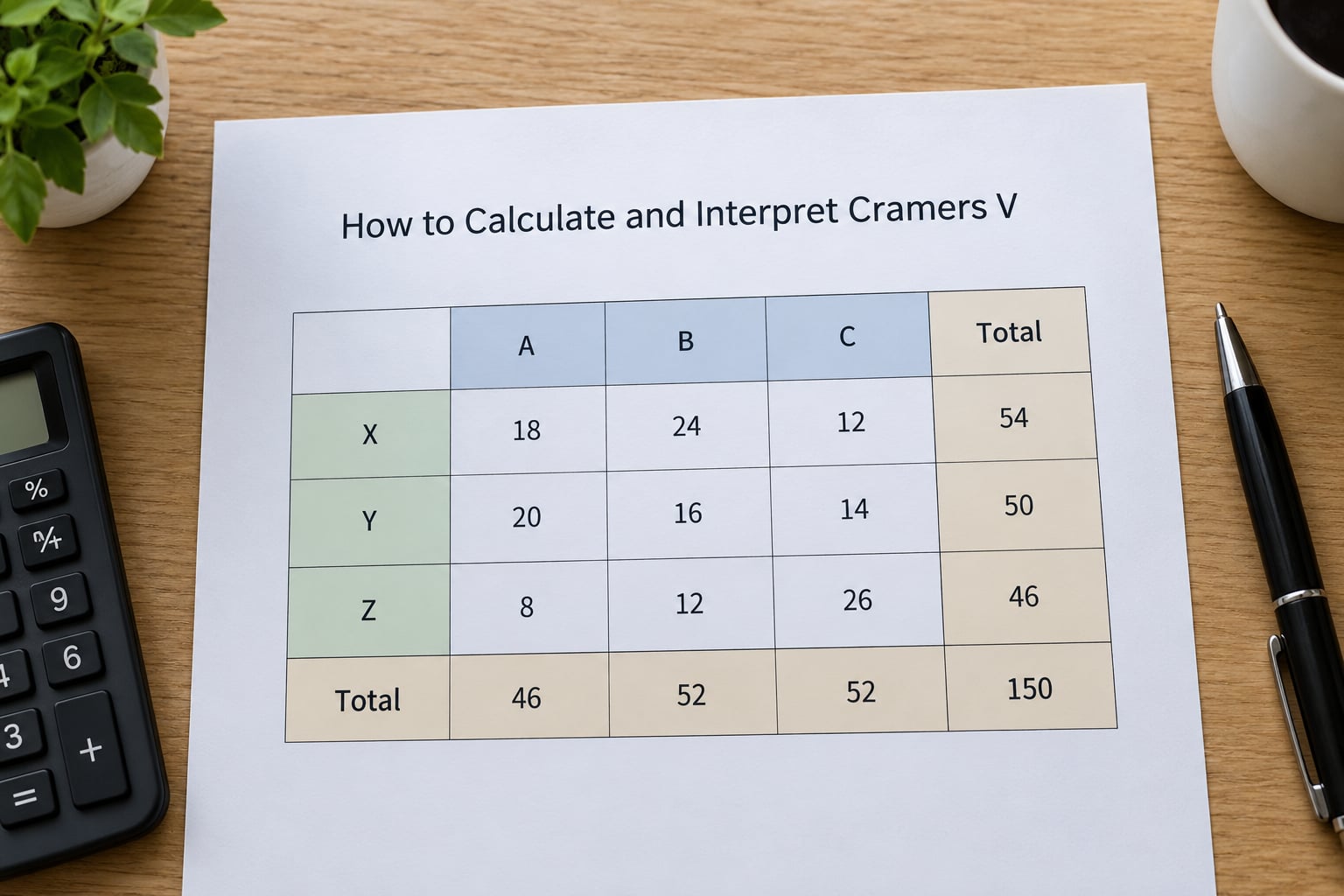
Cramér’s V is a normalized chi-square: it takes the chi-square statistic and rescales it to fall between 0 and 1, so tables of different sizes and different dimensions can be compared directly.

The formula is:

V = √[ χ² / ( n × ( min(r − 1, c − 1) ) ) ]

where χ² is the Pearson chi-square statistic, n is the total number of valid cases, and min(r − 1, c − 1) uses whichever dimension of the table is smaller after subtracting one. A 3×2 table gives you min(2, 1) = 1. A 4×4 table gives you min(3, 3) = 3.

Three things this number is not. It is not a correlation coefficient in the Pearson sense; it has no direction, no linear meaning, and no sign, and a value of 0.6 does not mean a predictable relationship the way r = 0.6 does. It is not a p-value and it cannot tell you whether the association is statistically significant. And it is not comparable across differently shaped tables unless you correct for the dimension, which the next sections cover.

Use it when both variables are categorical, when you want to state the strength of an association in a paper, and when you want to compare association strength across several tables built from different variables. Do not use it for ordinal data you intend to analyse with Spearman, and do not use it when one of your variables is continuous and uncategorised.

Cramer’s V and the phi coefficient are the same number for a 2×2 table, since min(r − 1, c − 1) equals 1 there. They diverge as soon as the table grows, and picking the wrong one is a common source of inflated results.

Consideration	Phi coefficient	Cramer’s V
Table size it handles	2×2 only	Any r × c table
Maximum possible value	1.0	1.0 on 2×2, lower on wider tables
Dimension correction	None	Divides by min(r − 1, c − 1)
Safe across studies	No, inflates with table size	Yes, once bias-corrected
Best use	Quick 2×2 reporting	Anything with 3+ categories

The pattern is consistent: V rises with n for a fixed population association, and shrinks as tables get larger for a fixed chi-square. Comparing a 0.30 from a 4×4 table to a 0.30 from a 2×2 table without correcting is the error that catches people out.

Step-by-Step

Step 1: Prepare the Contingency Table

Code each categorical variable as a labelled variable with no leftover numeric codes, then cross-tabulate them to get observed counts. The table here asks whether satisfaction level depends on how the customer made contact. The wording matters: “how they contacted us” has to mean the same thing in every record, or the counts mix different constructs.

Satisfaction	Online	In store	Row total
Very satisfied	48	27	75
Satisfied	36	24	60
Dissatisfied	16	24	40
Column total	100	75	175

The table is r = 3 rows by c = 2 columns. n = 175, from the grand total. Check that every category is meaningful before you go further: a row with two cases and a column with one case produce expected counts below 5, and the chi-square approximation stops being trustworthy.

Step 2: Calculate the Chi-Square Statistic

Expected count for each cell is the row total times the column total divided by n. For the very satisfied / online cell: (75 × 100) / 175 = 42.857. For very satisfied / in store: (75 × 75) / 175 = 32.143.

Work through the rest the same way:

Cell	Observed (O)	Expected (E)	(O − E)	(O − E)²/E
Very satisfied / Online	48	42.857	5.143	0.617
Very satisfied / In store	27	32.143	−5.143	0.823
Satisfied / Online	36	34.286	1.714	0.086
Satisfied / In store	24	25.714	−1.714	0.114
Dissatisfied / Online	16	22.857	−6.857	2.054
Dissatisfied / In store	24	17.143	6.857	2.738

Adding the last column gives χ² = 6.43. The cells driving that number are the dissatisfied row, where online contact produced fewer dissatisfied customers than independence would predict.

Do not stop here. A chi-square of 6.43 with df = 2 gives p = .040, which is significant at the .05 level, and the chi-square statistic grows with sample size. That is why the next step exists.

Step 3: Find the Sample Size and Degrees of Freedom

n is the grand total: 175 valid cases. If you excluded missing values, use the count that went into the chi-square, not your original sample size. Degrees of freedom are (r − 1)(c − 1), so here (3 − 1)(2 − 1) = 2.

For the Cramer’s V denominator, take the smaller of r − 1 and c − 1, which is min(2, 1) = 1. Keep these two numbers straight; confusing the degrees of freedom for the denominator term is the single most common arithmetic error in hand calculations.

Step 4: Calculate Cramers V

Substitute the values:

V = √[ 6.43 / ( 175 × 1 ) ] = √[ 6.43 / 175 ] = √0.0367 = 0.192

Round to two decimals for reporting: V = 0.19. The number sits between 0 and 1 as it always does, and it is a small association. Worth noting what the p-value said: p = .040, significant, while the effect is weak. Both statements are true, and you report both.

Step 5: Interpret the Effect Size

The fixed cut-offs most guides print are Cohen’s benchmarks for small tables: below 0.10 negligible, 0.10 to 0.30 weak, 0.30 to 0.50 moderate, above 0.50 strong. Our V of 0.19 falls in the weak band, which is consistent with the intuition that dissatisfied customers contact online slightly more than satisfied ones, but not dramatically.

Those benchmarks assume min(r − 1, c − 1) = 1. On larger tables, the maximum achievable V rises well above 0.5, so a V of 0.35 on a 5×5 table is not a moderate association. Cohen’s fix is to divide by the square root of min(r − 1, c − 1) before comparing against the thresholds. With 175 cases and df = 2 here, the correction factor is √1 = 1, so the bias-corrected value stays 0.19.

Read V as “how much the categories lean toward each other,” not as a percentage of anything. Report it alongside the chi-square statistic, its degrees of freedom, the p-value, and n, and describe the direction of the pattern in words so a reader knows which cells drive the number.

For an r × c table with more than one dimension, Cohen’s bias correction is V_corrected = V / √(min(r − 1, c − 1)). A common alternative is the Bergsma correction, which adjusts the chi-square itself for small-sample bias before the V is taken. Neither is mandatory, but if you report a raw V on a 5×5 table, say in a note that the uncorrected value was used.

People ask whether two Cramer’s V values from different samples differ meaningfully. There is no simple cutoff test built into the measure, and comparing two p-values does not answer it. Bootstrap both, or if you need a formal test, use a permutation approach that resamples the group labels and builds a null distribution of V values. With very large samples, tiny differences in V reach significance while staying irrelevant in practice, so the same caution about effect size versus significance applies to comparisons between V values.

How to Calculate and Interpret Cramers V in SPSS, R, and Stata

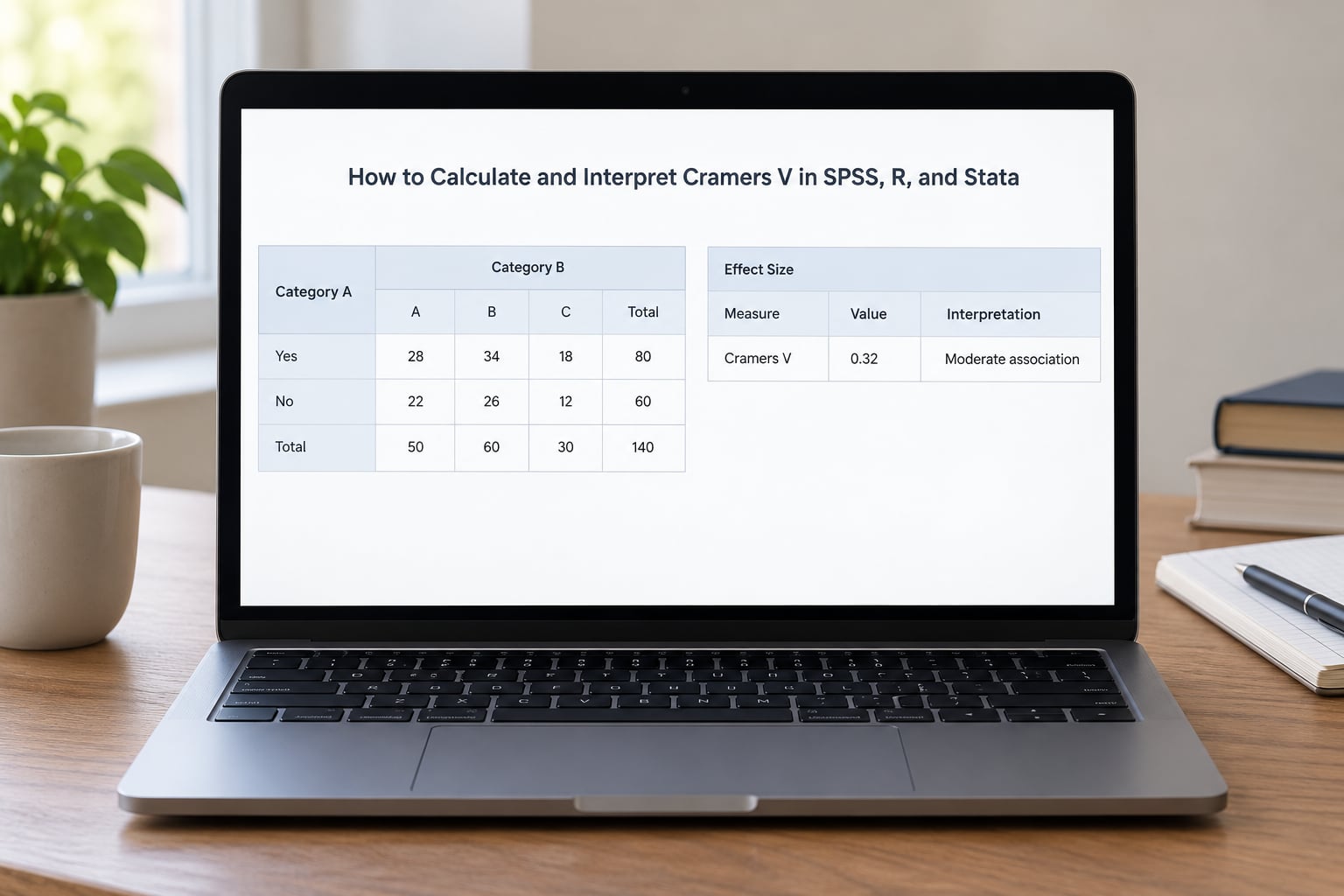
SPSS

Go to Analyze > Descriptive Statistics > Crosstabs. Put the row variable in Rows and the column variable in Columns, then click Statistics and tick Phi and Cramér’s V. SPSS prints both in the Symmetric Measures table along with the Approximate Significance column. With a 2×2 table, the Phi value equals Cramer’s V; on larger tables SPSS also offers a Bias-corrected row, which is the dimension-corrected version and the one to report if you want comparability across tables.

If your expected counts are low, the crosstab dialog will warn you. Fix that before reading the effect size.

R

Base R does not have a built-in Cramer’s V function, so it takes three lines. The chisq.test output includes the statistic and the parameter needed for the denominator.

t <- matrix(c(48, 27, 36, 24, 16, 24), nrow = 3, byrow = TRUE)
res <- chisq.test(t)
k <- min(dim(t)) - 1
V <- sqrt(unname(res$statistic) / (sum(t) * k))
V

The lsr package provides a cramersV() helper if you would rather not write it each time. For a confidence interval, bootstrap it: resample rows with replacement 1000 times, recompute V each time, and take the 2.5th and 97.5th percentiles.

Stata

Run tabulate satisfaction contact, chi2. For a 2-row table Stata prints Cramer’s V in the footer of the crosstab. On larger tables it does not, so capture the counts and compute it yourself:

tabulate satisfaction contact, chi2
matrix t = r(table)
local c2 = r(chi2)
local n = sum(`c2'[1, .])
local k = min(rowsof(`c2') - 1, colsof(`c2') - 1)
display sqrt(`c2' / (`n' * `k'))

The row total in r(table) gives you n and the matrix dimensions give you k, so the only extra piece is the chi-square from r(chi2).

Python and Excel

SciPy gives you everything in one call:

from scipy.stats import chi2_contingency
import numpy as np

table = np.array([[48, 27], [36, 24], [16, 24]])
chi2, p, dof, expected = chi2_contingency(table)
n = table.sum()
k = min(table.shape) - 1
V = np.sqrt(chi2 / (n * k))

In Excel without add-ins, use CHISQ.TEST on the two ranges to get the p-value, then convert it back to the statistic with CHISQ.INV.RT, and take the square root of that value divided by the grand total and k. If CHISQ.INV.RT returns an error for an extreme p-value, round the p-value to a few decimals first.

How to Report Cramers V in a Research Paper

APA 7 wants the chi-square test, its degrees of freedom, the p-value, and the effect size in the same sentence. Using our example:

A chi-square test showed an association between contact channel and satisfaction, χ²(2, N = 175) = 6.43, p = .040, Cramér’s V = 0.19. Dissatisfied customers were more likely to contact support online than satisfied customers were.

That final clause is doing real work. A bare effect size leaves the reader guessing which direction the relationship runs, and Cramér’s V cannot tell them. Fill-in template: “A chi-square test showed [a significant / a non-significant] association between [variable 1] and [variable 2], χ²([df], N = [n]) = [value], p = [value], Cramér’s V = [value].”

If you corrected for table bias, say so in a note, and report the corrected value rather than the raw one so readers do not have to guess which you used.

Do not italicise the V or write it with a leading zero omitted inconsistently across your tables. APA style keeps the leading zero for a statistic bounded between 0 and 1, and writes Cramér’s V with the accent or without it consistently. Check your journal’s style guide, since some drop the accent in the running text and keep it in the reference list.

One more habit worth building: state your table dimensions in the method or results section. “Contact channel (2 categories) by satisfaction (3 categories)” tells a reader enough to know which benchmark applies to your V without them having to reconstruct it.

Common Mistakes

Using (r − 1)(c − 1) as the denominator. The degrees of freedom and the Cramer’s V divisor are different numbers. For a 3×3 table, df = 4 but k = 2, so dividing by df halves your V.

Treating V as a correlation. It has no sign, no direction, and no linearity. Saying “a Cramér’s V of 0.6 means a strong relationship” without describing which cells are driving it leaves the finding uninterpretable.

Reading a weak V as a non-finding. With a large n you can get p < .001 on V = 0.07. The association exists and is trivially small, which is a completely different conclusion from no association, and usually the more useful one.

Ignoring the table dimensions. On a 6×6 table the maximum possible V is roughly 0.707, so the standard cut-offs understate strength. Apply Cohen’s correction before comparing.

Calculating on a table with tiny expected counts. If more than 20% of cells have expected values under 5, the chi-square approximation is unreliable and so is the V built on it. Merge the sparse categories, collect more data, or report the test as descriptive only.

Using percentages instead of counts. The formula needs frequencies. Percentages work only if every cell is scaled by the same factor and you multiply back to counts first.

Reporting V without n. Effect size grows more reliable as n grows, and a V of 0.30 from 40 cases is not the same claim as V = 0.30 from 4,000.

Collapsing categories to force a 2×2 table. It is tempting when phi looks cleaner, but merging categories to hit a shape destroys information and changes the question you were asking. Keep the original grouping if it has a defensible interpretation.

Assuming independence is the only assumption. Cramer’s V also assumes the two variables are sampled independently, each record falls in exactly one cell, and observations within the sample are independent of each other. Clustered or repeated data breaks that assumption, and the standard chi-square approximation no longer applies.

Citing a threshold as if it were a law. The cut-offs come from Cohen’s 1988 benchmarks and later critiques proposed different ones. Phrase it as “weak by common convention” rather than as a universal boundary.

Frequently Asked Questions

Conclusion

Start by building the contingency table from counts, checking that every expected cell is large enough to trust. Run the chi-square test, note the statistic, n, and degrees of freedom, then divide by n times min(r − 1, c − 1) and take the square root.

Report that V next to the p-value, not instead of it, and correct for table size when you compare effect sizes across different tables. The number tells you how strong the association is; your prose has to tell the reader what the association looks like.