How to Read a Normal Distribution Curve 2026: Simple Guide

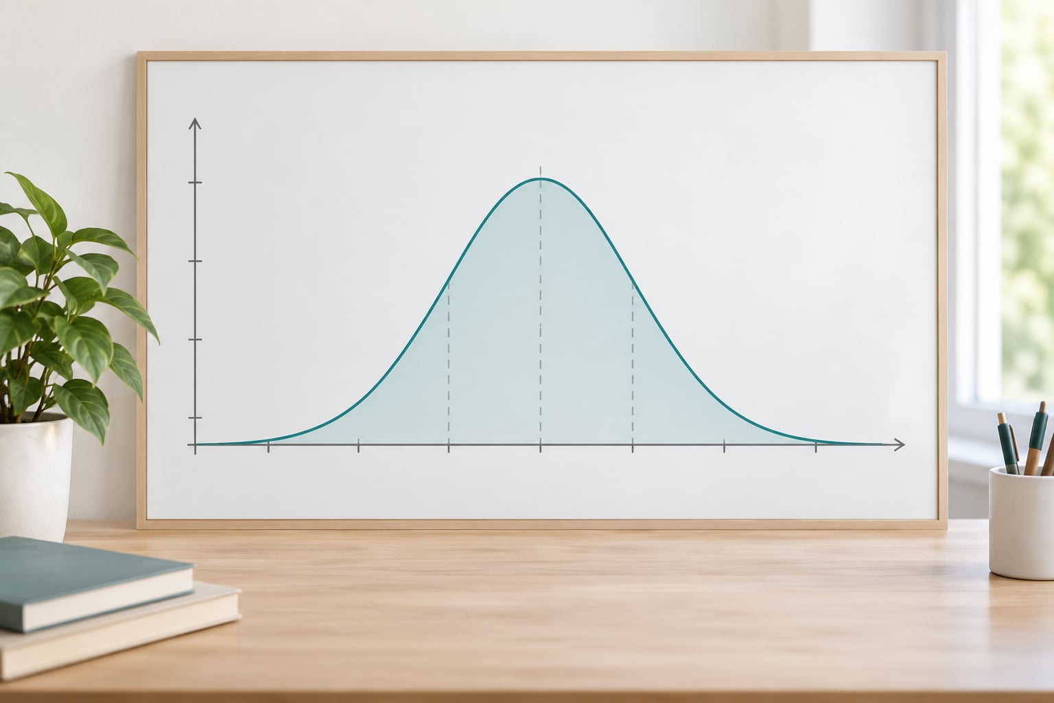
A normal distribution curve is a symmetric, bell-shaped probability graph in which most values cluster around the mean at the centre and values taper off evenly in both directions, with the total area under the curve equal to 1. Reading it comes down to four moves: find the mean, count standard deviations away from it, shade the region you care about, and read that region’s area as a percentage. Everything else on the page, including z-scores, percentiles and confidence intervals, is a shortcut built from those four steps.

If you are working through exam questions that hand you probabilities and ask for the mean and standard deviation, this guide works backwards too. There is a worked example for that near the end.

Table of Contents

1. 1What Does a Normal Distribution Curve Show?
2. 2Key characteristics of a normal distribution curve
3. 3How to Read a Normal Distribution Curve Step by Step
4. 4What Do the Mean and Standard Deviation Tell You?
5. 5How Do I Interpret the Area Under the Curve?
6. 6Reading a normal distribution curve as area
7. 7What Is a Z-Score on a Normal Distribution Curve?
8. 8How to Read a Standard Normal Curve
9. 9How Do You Know If Data Are Approximately Normal?
10. 10Common Examples of Reading a Normal Distribution
11. 11Frequently Asked Questions
12. 12What is the z-score for a 95% normal distribution?
13. 13How do I use the 68-95-99.7 rule?
14. 14How do I interpret a z-score?
15. 15How do I read a distribution graph?
16. 16Based on the empirical rule, how many standard deviations of the mean do 95% of data points fall within?
17. 17Does a z-score require a normal distribution?

What Does a Normal Distribution Curve Show?

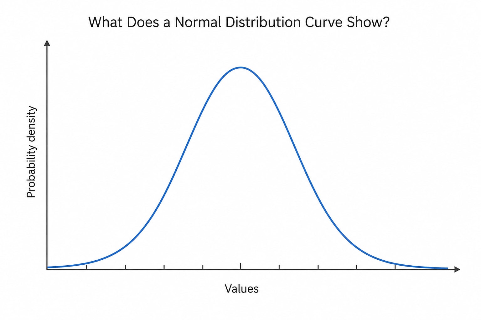
Two axes do all the work. The horizontal axis lists the values your variable actually takes, in the units you recorded them, such as test scores, heights in centimetres or reaction times in milliseconds. The vertical axis shows probability density, which is a rate rather than a probability at that exact point.

That distinction trips up nearly everyone at first. For a continuous variable like height, the probability of being exactly 172.4 cm is effectively zero, because a continuous measurement can land on any value. What you read instead is the height of the curve at 172.4 as a density, and it becomes a probability only when you measure the area across an interval. A width of 2 cm times a height of 0.3 per cm gives an area of 0.6.

Key characteristics of a normal distribution curve

• Symmetry. The left and right halves are mirror images of each other.
• Mean = median = mode. All three land on the peak at the centre.
• Two governing values. The mean (μ, mu) sets the position and the standard deviation (σ, sigma) sets the spread. Nothing else is needed.
• Asymptotic tails. The curve approaches the horizontal axis and gets closer without ever touching it.
• Total area = 1. Every observation that could ever occur is somewhere under the curve, so the shares always add to 100%.
• No corners. A normal curve is smooth everywhere, which is why it suits measurements that average out many small influences.

One point on terminology, since it comes up constantly on stats forums. A bell curve is the shape. A normal distribution is the specific probability density function that produces that shape, and not every bell-shaped thing is one. Skewed data and two-peaked data both look vaguely bell-ish, and both break the 68-95-99.7 arithmetic you are about to do.

How to Read a Normal Distribution Curve Step by Step

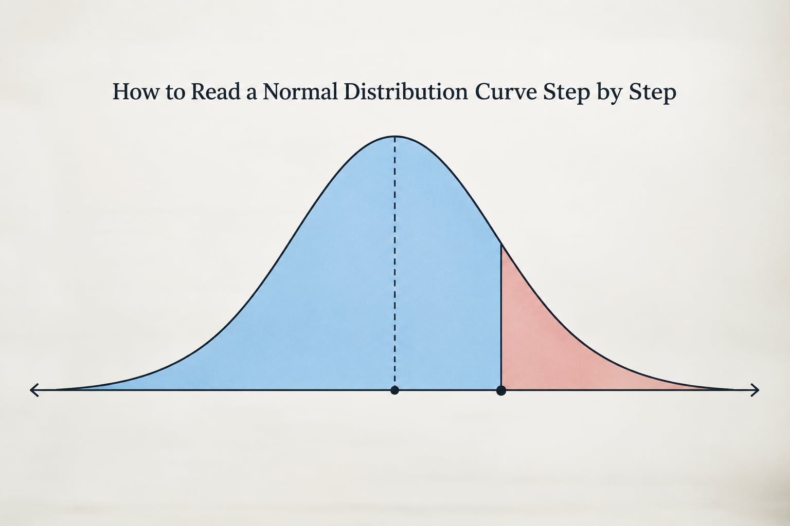
Six steps, the same every time. I have walked students through this sequence on paper more times than I can count, and the mistakes almost always come from skipping step 3.

1. Identify the variable and its units. Write down what the horizontal axis measures before touching the curve.
2. Find the centre. Locate μ on the horizontal axis. The peak of the curve sits directly above it.
3. Mark the standard deviations. Place μ ± 1σ, μ ± 2σ and μ ± 3σ on the axis and draw vertical guides up to the curve.
4. Place your value. Drop a line from the score, measurement or cut-off you care about to the axis.
5. Shade the region. Colour in the area your question is about: to the left of your value, to the right, or between two values.
6. Read the area. Convert the shaded fraction to a percentage, then multiply by your sample size to get a head count.

A worked example carries the last three steps. Suppose exam scores have a mean of 72 and a standard deviation of 8, so the marks sit at 64, 72, 80, 88 and 96 for one, two and three standard deviations. A score of 88 sits exactly at μ + 2σ, so about 2.5% of scores fall above it and about 97.5% fall below it. In a class of 40, that is roughly one student above 88 and 39 below.

The count matters more than people expect. A percentage with no denominator tells you nothing about your own data, and converting at the end is where curve-based grading goes wrong when it is done by eye instead of by area.

What Do the Mean and Standard Deviation Tell You?

The mean is the balance point and the standard deviation is the typical distance from it. Roughly two-thirds of values fall within one standard deviation of the mean, and the rest sit progressively further out.

Because only μ and σ define the curve, you can predict what any change to them does before you draw anything.

Change	What the curve does	What it means
Mean rises from 72 to 80, σ unchanged	The whole curve slides right, same shape and same height	Scores shifted up; nothing got more consistent
Standard deviation rises from 8 to 12	The curve spreads wider and peaks lower	The same data now look more variable
Standard deviation falls from 12 to 8	The curve narrows and peaks higher	Performance is more tightly clustered

A common confusion here: sigma controls width, not height. A taller peak does not mean more data. The area stays at 1 either way, so a narrow curve is a shorter, fatter-looking bell and a wide curve is a flatter one.

How Do I Interpret the Area Under the Curve?

Reading a normal distribution curve as area

Area is probability, and it only makes sense over an interval. That is why “the probability of a score being 88” is a trick question on a continuous scale, while “the probability of a score being below 88” is perfectly well defined.

Reading a normal distribution curve mostly means trusting the empirical rule, also called the 68-95-99.7 rule. It is an approximation, not an identity, and it is close enough for most descriptive work and for catching problems early.

Region	Span from the mean	Share of the data	Left outside	Right outside
One standard deviation	μ − 1σ to μ + 1σ	About 68%	About 16%	About 16%
Two standard deviations	μ − 2σ to μ + 2σ	About 95%	About 2.5%	About 2.5%
Three standard deviations	μ − 3σ to μ + 3σ	About 99.7%	About 0.15%	About 0.15%

Those tail figures are the practical payoff. If your right tail is 2.5%, you have a one-in-forty chance of scoring above a threshold, which is exactly how a 95% confidence interval and a 5% significance level are built. It also gives you a rough outlier rule: values past 3σ are rare enough to warrant a look at the source data.

What Is a Z-Score on a Normal Distribution Curve?

A z-score is the number of standard deviations a value sits from the mean. The formula is short:

z = (x − μ) ÷ σ

It answers “how unusual is this, in units of spread”, which is why it works across subjects. A score of 88 in an exam with a mean of 72 and a standard deviation of 8 gives z = (88 − 72) ÷ 8 = 2. A time of 12 seconds on a task with a mean of 10 and a standard deviation of 2 also gives z = 2. Different scales, same statement about relative standing.

• z = 0 is the mean itself, at the 50th percentile.
• z = +1 is one standard deviation above, around the 84th percentile.
• z = −1.5 is one and a half below, around the 7th percentile.
• z = +3 is three above, above roughly 99.85% of values.

The sign simply tells you the direction. That is the whole thing, and once it clicks, z-scores stop being a separate topic and become the step-by-step method above with the units swapped out.

How to Read a Standard Normal Curve

The standard normal curve is the same shape shifted to mean 0 and scaled to a standard deviation of 1. Every measurement problem gets converted onto it before any probability is looked up, so the horizontal axis is just a z-axis running from about −3 to +3.

To read a probability from it, find your z on the axis, walk vertically to the curve, then follow down to the table or calculator that gives the cumulative area from the far left tail up to that point.

Take z = 1.25. On a standard normal table, find 1.25 in the row and the second decimal column. The cumulative area is 0.8944, so about 89.4% of values fall below a z of 1.25 and about 10.6% fall above it. Between 0 and 1.25 lies 0.3944 of the curve, or 39.4%. Between −1.25 and +1.25 the share is 0.7888, or about 79%.

In software the same lookups have names worth knowing. In R, pnorm(1.25) returns the cumulative area and norm.ppf(0.8944) works the other way, turning a probability back into a z. In Excel, NORM.S.DIST(1.25, TRUE) gives the cumulative value and NORM.INV(0.8944, 0, 1) inverts it. In SPSS, Explore then Plots then Histogram with the Normal curve checkbox overlays the fitted curve on your data so you can compare shape by eye.

How Do You Know If Data Are Approximately Normal?

Start with a histogram. You want one clear peak, roughly equal spread on both sides, and no long tail dragging off in one direction. Slight lumps in the middle are fine and often just sample noise.

A Q-Q plot, which plots your sorted values against the values a perfect normal would produce, gives a sharper answer. Points hugging a straight diagonal line mean the shape is close to normal; a visible S-bend signals skewness, and points bending away at both ends signal heavy tails.

Then check the summary statistics. Skewness near zero and excess kurtosis near zero are what a normal distribution predicts. A strong positive skewness number, or a bimodality coefficient well above 0.555, is a warning that you are looking at two overlapping groups rather than one population.

Formal tests such as Shapiro-Wilk give a p-value, and here the caution matters. A small p-value is evidence against normality. A large p-value is not proof of normality, because those tests have little power with small samples and almost never reject a near-normal sample. Treat the plot and the substantive knowledge of your data as the primary evidence and the test as a supporting one.

Common Examples of Reading a Normal Distribution

The curve shows up in academic work more than most people expect. Each of these needs the same four numbers identified: mean, standard deviation, the interval of interest, and the percentage that falls inside it.

Exam scores to a percentile. A cohort averages 68 with a standard deviation of 11. A score of 79 is 1σ above the mean, so about 84% of the group scored lower. In a class of 120, that is roughly 101 students below it.

Heights. Adult heights in a population average near 171 cm with a standard deviation of about 7 cm for women and 8 cm for men. Between 157 cm and 185 cm for women is μ ± 2σ, which by the empirical rule covers about 95% of people.

Measurement error. A balance that reads a true mass of 5 kg with a standard deviation of 20 g produces readings that cluster near 5 kg and thin out on both sides. Outlier rules applied to repeated measurements work because the error distribution is roughly symmetric.

Sampling distributions. The central limit theorem says the distribution of sample means approaches normal as sample size grows, even when the raw data are not normal. That is why a confidence interval for a mean gets tighter as n rises: the standard error shrinks and the curve narrows.

Solving backwards from probabilities. When you are given P(X < 20) = 0.50 and P(X < 26) = 0.9772, work in reverse. The first statement says 20 sits at the mean, because half the area always falls below the mean, so μ = 20. The second says 26 sits at about 2σ, since 97.72% of a normal distribution falls below 2σ, so σ = 3. This reverse direction is the most common exam variant and the one most tutorials skip.

Grading on a curve. Converting each mark to a z-score and then to a percentile is defensible only when the cohort really is roughly normal. Check the histogram first. Two peaks usually mean two ability groups plus a course policy you cannot infer from the data, and a curve fitted to it will hand out grades that look precise and are not.

Data that should not be forced onto this curve at all: bounded scales such as 1 to 5 Likert items, anything with a ceiling or floor, skewed income or waiting-time data, and small samples under roughly 30 observations.

Frequently Asked Questions

Do one thing first: take a single number you care about, work out its z-score, and then read the percentile off a standard normal table before touching any software. Once that one conversion is automatic, the whole curve stops being a picture and becomes a calculator.