How to Transform Skewed Data for Analysis (October 2026)

To transform skewed data for analysis, first confirm the skew with a histogram, a box plot and a skewness coefficient, then apply the least disruptive method that fixes it: square root for moderate right skew, log for severe right skew, cube root or Yeo-Johnson when negatives are present, and reflection before anything else when the tail points left. Then you recheck the distribution, run the analysis, and document what you did. It takes about 20 minutes once you know which method fits.

Most people get this wrong at step two, not step one. They transform first and diagnose later, or they delete the handful of extreme cases that were creating the skew in the first place. Both produce a tidy histogram and a weaker study.

This guide walks through the full sequence: diagnosing skewness, matching it to a method, running that method in SPSS, R or Python, verifying the result, and writing it up so a reader can follow.

Table of Contents

1. 1What You Need
2. 2Step-by-Step
3. 3Step 1: Inspect the Distribution and Confirm Skewness
4. 4Step 2: Choose the Right Transformation
5. 5Step 3: Create a New Transformed Variable
6. 6Step 4: Recheck the Distribution and Statistical Assumptions
7. 7Step 5: Run the Intended Analysis and Compare Results
8. 8Step 6: Document and Report the Transformation
9. 9Common Mistakes
10. 10Frequently Asked Questions
11. 11What is the best way to transform skewed data for analysis?
12. 12Should I use a square-root, log, or Box-Cox transformation?
13. 13Can I transform data with zero or negative values?
14. 14How do I know if a transformation fixed the skewness?
15. 15Should I analyze the original data or the transformed data?
16. 16How do I report a data transformation in a research paper?
17. 17Conclusion

What You Need

Before touching anything, make an untouched copy of your raw data. You will want the original scale later when you back-transform results, and a transformation you cannot undo is a transformation you cannot report properly.

You also need:

• The variable’s type and role. Continuous measurement, count, ordinal score or category. Transformations apply to continuous and count variables; a category label like “Region 3” has no numeric meaning to transform.
• A check for zeros and negative values. This decides your method list more than anything else, and skipping it is why log transformations produce a column of missing values.
• Statistical software. SPSS through Transform menu, R, or Python with pandas, scipy and scikit-learn. Any of the three runs every method in this guide.
• A histogram, a box plot and descriptive statistics for the variable, plus the skewness coefficient.
• Your planned analysis. A transformation is only justified by the assumption it repairs. A t-test on raw residuals needs normality; a Mann-Whitney test does not, and transforming for it is wasted work.

Step-by-Step

Step 1: Inspect the Distribution and Confirm Skewness

Start with a histogram, then a box plot. The histogram shows the shape of the bulk; the box plot shows the tail length and any outliers as separate points, which is often clearer.

Next compare the mean and the median. If the mean sits noticeably above the median, the tail runs to the right and the data is right-skewed, also called positively skewed. If the mean sits below the median, the tail runs left and the data is left-skewed.

Then read the skewness coefficient, the standardized third moment of the distribution. Zero means symmetric, positive means right-skewed, negative means left-skewed.

Skewness value	What it means	What to do
Between -0.5 and 0.5	Close to symmetric	Leave it alone
Between 0.5 and 0.75 either side	Mild to moderate skew	Check the residuals, not just the raw variable
Beyond 0.75	Noticeable skew, the usual trigger point	Transform and verify
Beyond 1.5	Severe skew, a few extreme values often drive it	Investigate those cases before transforming

One warning about thresholds, because it confuses almost everyone. Different software reports skewness on different scales. SPSS reports the raw moment coefficient, typically around -1 to +1 in practice. SPSS also reports a standardized skewness that divides the coefficient by its standard error, which is why those numbers sit roughly inside -3 to +3 and grow with sample size: a standardized value of 2 in a sample of 5,000 tells you far less than a raw value of 1.2 does. R’s skewness() and pandas’ .skew() use the raw coefficient, so the familiar 0.75 rule of thumb applies directly there.

So if your SPSS output says “Skewness, Std. Error = 0.30” and “Skewness = 0.90”, you have a moderate-to-clear right skew. If it says “Skewness = 0.20” and “Std. Error = 0.03”, your standardized value is about 6.7 and looks alarming, but the actual shape is close to symmetric and the large number is a small standard error. Always judge the raw coefficient and look at the plot.

Step 2: Choose the Right Transformation

Match the method to three things: which way the tail points, whether zeros or negatives exist, and how hard you need to pull the shape back.

Transformation	Best for	Zeros	Negatives	Strength
Square root	Counts, frequencies, moderate right skew	Allowed	Not allowed	Gentle
Log (base 10 or natural)	Severe right skew, income, revenue, ratios	Not allowed	Not allowed	Strong
Log(x + 1) or log1p	Right skew with zeros present	Allowed	Not allowed	Strong
Cube root	Right skew, and you must keep negatives	Allowed	Allowed	Moderate
Box-Cox	Strictly positive right-skewed data	Not allowed	Not allowed	Strong, lambda is fitted
Yeo-Johnson	Mixed signs, or any zero	Allowed	Allowed	Strong, lambda is fitted
Reflection then log or square root	Left-skewed data	After reflection	After reflection	Strong
Square or exponential	Mild left skew on a bounded scale	Allowed	Allowed	Gentle

On Box-Cox and Yeo-Johnson: both estimate a power parameter, called lambda, that decides the strength of the transformation. Lambda of 1 is no change, 0 is the log, 0.5 is the square root, and -1 is the reciprocal. Box-Cox needs strictly positive data. Yeo-Johnson handles zeros and negatives, which is why it is the safer default in survey and finance work where you cannot guarantee positivity.

For left-skewed data, most published guides say nothing at all, which is why so many people end up logging a variable that needs the opposite treatment. The fix is reflection: reverse the scale so the left tail becomes a right tail, then apply a right-skew method to the reversed variable. With Likert items scored 1 to 5, the usual constant is 6, so a reversed item is 6 minus the original. Composite survey scores are left-skewed more often than analysts expect, because respondents cluster at the top of the scale.

Mild left skew on a bounded scale can often be fixed with the square or exponential function alone, no reflection required, since both push values upward and open out the compressed left side.

In SPSS, the whole method lives in one dialog. Go to Transform > Compute Variable, type the target variable name, click the function group, and pick the function.

• LOG10(x) for a log base 10, LN(x) for the natural log. Add a constant inside the brackets for zeros, so LOG10(income + 1).
• SQRT(x) for the square root.
• EXP(x) for the exponential, one of the left-skew options.
• RANK(x) or NORMAL(x) if you want percentile ranks or a normal score instead.

Left skew in SPSS has no one-click menu. Use Compute Variable with a reflection constant, for example 6 minus the original item, then apply LOG10 or SQRT to that new variable.

The same methods in R and Python:

# R
df$log_income  <- log(df$income)
df$log1p_income <- log1p(df$income)
df$sqrt_count   <- sqrt(df$count)
df$cbrt_net    <- sign(df$net) * abs(df$net)^(1/3)
df$reversed    <- 6 - df$likert_item
df$bc  <- MASS::boxCox(lm(y ~ x, data = df))
df$yj  <- car::yeojohnson(y ~ x, data = df)

# Python
df["log_income"]    = np.log(df["income"])
df["log1p_income"]  = np.log1p(df["income"])
df["sqrt_count"]    = np.sqrt(df["count"])
df["cbrt_net"]      = np.sign(df["net"]) * np.abs(df["net"]) ** (1/3)
df["reversed"]      = 6 - df["likert_item"]
from scipy import stats
bc = stats.boxcox(df["income"])
yj = stats.yeojohnson(df["net"])
from sklearn.preprocessing import PowerTransformer
pt = PowerTransformer(method="yeo-johnson")

Step 3: Create a New Transformed Variable

Never overwrite the original. Add a new variable alongside it, named something like log_income, so you can put both in the same model and compare results later.

Then check for undefined results before moving on. Look for missing values that appeared only in the new variable, which means the function returned something invalid for at least one row. The usual causes are zeros or negatives meeting a log or square root, and negative values meeting an even root.

Confirm the ordering of observations is preserved: a transformation changes values, never which row each value belongs to. If you used Box-Cox or Yeo-Johnson, record the fitted lambda, because you need it to reverse the transformation later.

Step 4: Recheck the Distribution and Statistical Assumptions

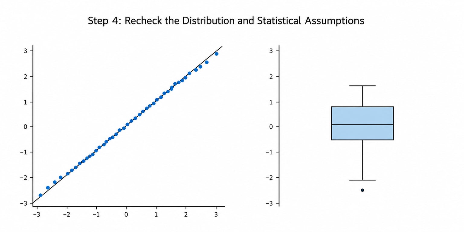
Plot the transformed variable the same way you plotted the original: histogram, box plot, and a Q-Q plot against a normal reference line. The Q-Q plot is the real test, because it answers whether the points sit near the diagonal rather than whether the histogram merely looks rounder.

Recompute the skewness coefficient and compare it to the original. A right-skewed income variable at 1.95 that drops to 0.13 after logging is a clear success. A move from 1.95 to 1.20 tells you the method was too gentle and you should go further.

Then run the assumption tests your planned analysis actually needs:

• Shapiro-Wilk for normality of a single variable. R: shapiro.test(x). In SPSS, Analyze > Descriptive Statistics > Explore, then request the normality test.
• Kolmogorov-Smirnov as a second opinion, and because it is what SPSS prints by default with Lilliefors correction.
• Residuals, not raw values. This is the step students skip. A t-test or linear regression needs normally distributed residuals, and a skewed raw variable often produces perfectly normal residuals. Plot residuals after fitting the model with the untransformed variable; if they look fine, stop.
• Levene’s test or a residual-versus-fitted plot for homoscedasticity. Transforming the response often stabilizes spread, which is half the reason it works.

With large samples, tests will detect deviations that do not matter in practice. A significant Shapiro-Wilk result on 2,000 cases can coexist with a p-value of 0.72 and perfectly usable results. Look at the effect size of the skew, not just the p-value.

Step 5: Run the Intended Analysis and Compare Results

Run the analysis twice: once on the original variable, once on the transformed one. Comparing them is the only way to know whether the transformation changed your conclusion or just your histogram.

Compare the estimates, the standard errors, the confidence intervals and the model fit. If the direction and significance of every coefficient hold steady and the residuals improve, the transformation did its job. If a coefficient flips sign or a p-value swings across 0.05, investigate before reporting anything.

Then decide how to interpret the result, and this depends on whether you transformed the response variable or a predictor. When you transform the response, your estimates are on the transformed scale. A log model gives you a multiplicative reading: exponentiate the coefficient to get a percent change, so a coefficient of 0.30 means roughly a 35 percent increase. When you transform a predictor, the model is non-linear in the original units and the coefficient no longer has a clean per-unit meaning.

To get results back on the original scale, back-transform. For a log model, exponentiate the coefficient and the confidence limits together. For a square root model, square the estimate, and add back any offset constant you used.

Also keep in mind when not to transform at all. This comes up constantly on statistics forums, and the honest answer is that transformation is a blunt instrument. A generalized linear model with a log link or a Poisson distribution handles right-skewed counts directly, without touching your data. Nonparametric tests such as Mann-Whitney or Kruskal-Wallis do not assume normality in the first place. Bootstrapping gives you valid confidence intervals from the raw data without assuming any shape, and bootstrapping is repeatedly recommended on those forums for exactly this reason. Robust standard errors correct the inference while leaving your variables in real units. If you have a credible alternative, use it rather than transforming by reflex.

Step 6: Document and Report the Transformation

Report the decision, not just the result. A reviewer needs to know the original shape, the method, why you chose it, and what the evidence looked like afterwards.

A complete report covers:

• The original distribution and its skewness value, with the convention you used.
• The assumption the transformation was repairing, and which analysis needed it.
• The transformation applied, written out as a formula.
• Any offset constant, such as log(x + 1), and why it was needed.
• The transformed skewness value and the normality test result afterwards.
• How you interpret the estimates, including any back-transformation.
• Whether you checked outliers first, and what you concluded.

A sentence that covers it: “Income was strongly right-skewed (skewness = 1.94, n = 412), which violated the normality assumption for the planned one-way ANOVA. A base-10 logarithmic transformation reduced the skewness to 0.13 (Shapiro-Wilk p = .21); one respondent reporting zero income was handled with log10(x + 1). A sensitivity analysis on the untransformed variable produced the same pattern of results.”

Common Mistakes

Transforming a categorical variable. Group codes and labels have no interval meaning, so transforming them is meaningless. Transform only continuous and count variables.

Applying a log to zeros or negatives. Both return undefined values, and your new variable fills with missing data. Use log1p, log(x + 1), or switch to cube root or Yeo-Johnson. Check for zeros before you choose, not after.

Transforming the grouping variable. The independent variable that splits your groups must stay in its original form, or the group difference you are trying to measure disappears.

Transforming every variable automatically. Feature-engineering pipelines often do this by reflex. A categorical flag, a bounded score and a variable that is already normal gain nothing and lose interpretability.

Deleting outliers instead of investigating them. A skew of 2 driven by three data-entry errors is an error problem, not a distribution problem. Fix the errors, then reassess. If the extreme values are genuine, keep them and consider winsorizing or a robust method rather than deletion.

Mixing skewness conventions. Comparing an SPSS standardized value of 2 against the 0.75 rule of thumb leads to transforming data that never needed it. State which coefficient you are quoting.

Showing only the improved histogram. Report the before and after numbers and the Q-Q plot. The plot is what convinces a reviewer.

Applying one transformation across a train and test split inconsistently. If you fit a Box-Cox or Yeo-Johnson lambda on your training data, you must reuse that same lambda on any future data. Refitting on new data silently changes the scale and breaks the model outside your sample.

Forgetting the offset constant at interpretation time. If you modelled log10(x + 1), the back-transform is 10 to the power of the estimate, minus 1. Skipping that minus one overstates every prediction.

Frequently Asked Questions

Conclusion

To transform skewed data for analysis, do three things in this order. Look at the distribution and confirm which way the tail points. Check for zeros, negatives and outliers, because those decide whether a log is even legal. Then choose the least disruptive method that fixes the documented problem, and verify it with a Q-Q plot and a second skewness number before you write a single word about your results.