
To check skewness and kurtosis values, you ask your software for two summary numbers and compare them against a reference point: skewness of 0 means the distribution is symmetric, and kurtosis of 0 means it is normal-shaped. In SPSS that takes about a minute through Analyze > Descriptive Statistics > Frequencies. Excel, R and Python all return the same two numbers too, so the software is not the hard part. Reading them is.
This guide covers the exact clicks in SPSS, the equivalent commands in Excel, R and Python, the bands most researchers use to interpret the output, and what to do when your values fall outside them. It takes roughly 10 minutes end to end once your data file is open.
Table of Contents
- 1What You Need
- 2The variable has to be continuous and numeric
- 3Mind the sample size
- 4Decide how missing values are handled
- 5Step-by-Step: How to Check Skewness and Kurtosis Values in SPSS
- 6Step 1: Prepare the variable for analysis
- 7Step 2: Run the skewness and kurtosis test
- 8Step 3: Interpret skewness and kurtosis values
- 9Step 4: Check the shape with a histogram
- 10Step 5: Use a normality test as supporting evidence
- 11Step 6: Record and act on the results
- 12Common Mistakes
- 13Frequently Asked Questions
- 14What are acceptable skewness and kurtosis values?
- 15Should I use both skewness and kurtosis?
- 16How do I find skewness and kurtosis in SPSS?
- 17Is a normality test required after checking skewness and kurtosis?
- 18What should I do if my data are not normally distributed?
- 19Can skewness or kurtosis be fixed by deleting outliers?
- 20Conclusion
What You Need
You need three things: your data file loaded, a working definition of which variable you are checking, and enough cases that the numbers mean something. Everything else follows from that.
The variable has to be continuous and numeric
Skewness and kurtosis describe the shape of a continuous distribution. A satisfaction score from 1 to 5, a salary figure, a test mark and a regression residual all qualify. A gender code, a region label or a yes/no flag does not. Running the test on a coded categorical variable gives you a number, but it describes something meaningless.
In the SPSS Variable View, check the Measure column for the variable. It should read Scale. Nominal and Ordinal variables need a different approach entirely, usually frequencies and percentages rather than shape statistics.
Mind the sample size
Below about 50 cases, every dataset looks skewed, because a handful of points drags the tail. In that range, treat the values as a rough description rather than a gate. Above 50, a skewness past 1 in each direction is worth acting on. Above 200, reviewers start expecting a written justification for anything extreme.
Decide how missing values are handled
SPSS excludes missing values by default, and that is almost always what you want. What trips people up is running Frequencies on one variable and Descriptives on another and getting slightly different numbers for the same data. The two procedures handle weighting, missing values and the bias correction differently, so small differences are normal, not a bug.
Step-by-Step: How to Check Skewness and Kurtosis Values in SPSS
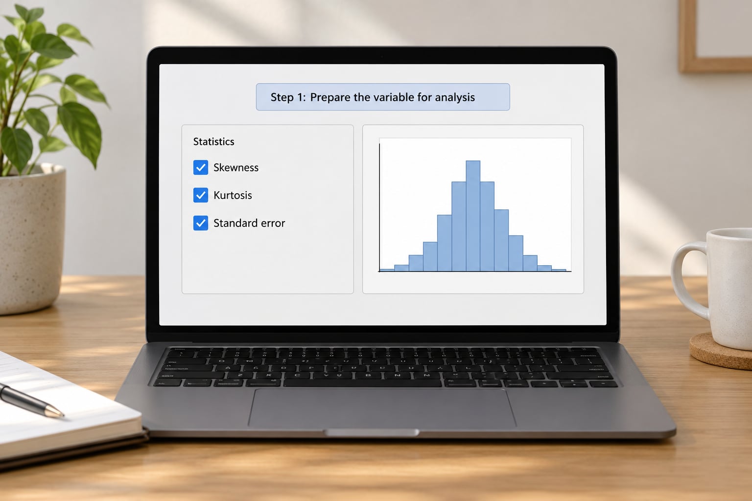
Step 1: Prepare the variable for analysis
Open the data file, then go to Variable View and confirm the target variable is typed as Numeric with no decimal comma or text in the cells. Text sneaks in when someone types a dash for a missing response, and SPSS reads that whole cell as missing rather than as a number.
Next, look at the Missing column. If you set a discrete missing value such as 9 for “did not answer”, the default system-missing handling still leaves it in the calculation unless you use Analyze > Descriptive Statistics > Frequencies and uncheck Values are labels, or you recode 9 as a user-missing value first. Getting this wrong quietly shrinks your effective sample.
Run a quick frequency table on the variable and glance at the minimum, maximum and spread. Values that are all identical produce a skewness and kurtosis of zero by default, which looks like a perfect normal distribution and means nothing.
Step 2: Run the skewness and kurtosis test
This is the click path most people are looking for. In SPSS, follow these steps in order:
- Open the menu Analyze.
- Choose Descriptive Statistics, then Frequencies.
- Move your variable from the left-hand variable list into the Variable(s) box on the right.
- Click the Statistics button on the dialog box.
- Tick Skewness and Kurtosis in the list of frequency statistics.
- Tick Std. Error if it is not already selected. This adds the standard error columns, which you want.
- Click Continue, then OK.
The output appears in the Output Viewer as a Frequencies table. The last two rows on the right of that table give you the values, and immediately beside them sit their standard errors. Those two extra columns are the most useful part of the table and the one most people skip.
To standardize, divide the skewness by its standard error. A ratio between minus 1 and 1 is comfortable, beyond 2 is a real departure from symmetry, and beyond 3 is severe. Do the same with kurtosis and its standard error. This ratio adjusts automatically for sample size, which is why it beats a fixed cutoff.
The other three packages do the same job in one line:
| Software | Command | What it returns |
|---|---|---|
| SPSS | Analyze > Descriptive Statistics > Frequencies > Statistics | Skewness, Kurtosis, both Std. Errors |
| Excel | =SKEW(A1:A100) and =KURT(A1:A100) | Skewness and excess kurtosis |
| R | e1071::skewness(x), e1071::kurtosis(x) | Skewness and excess kurtosis |
| Python (pandas) | df.skew(), df.kurt() | Skewness and excess kurtosis |
One important detail in that table: SPSS, R, pandas and Excel all report excess kurtosis, where a normal distribution scores 0. If you have ever worked from a textbook saying a normal distribution has kurtosis of 3, that is the raw Pearson value, and subtracting 3 converts one to the other. It is the single most common source of confusion in this topic.
In Excel, SKEW and KURT need no add-in. The Analysis ToolPak route gives you a formatted output table instead: File > Options > Add-ins > Manage Excel Add-ins > Go > tick Analysis ToolPak, then Data > Data Analysis > Descriptive Statistics, and tick Summary statistics. Leave the other boxes unticked or the output gets cluttered.
Step 3: Interpret skewness and kurtosis values
Start with skewness. Zero means the left and right sides mirror each other. Positive values mean the tail stretches to the right, which is what income, house prices and most right-censored measurements do; the mean then sits above the median. Negative values mean a long left tail, common when a score is bounded below and a few respondents hit the floor.
Kurtosis reads differently. It describes how heavy the tails are and how sharp the peak is, not how far the data spread overall. Excess kurtosis of 0 is normal-shaped. Positive values mean leptokurtic: a sharp peak with heavy tails, which is what you see when a few extreme values sit in a narrow distribution. Negative values mean platykurtic: a flat top and light tails, often the signature of scores that cluster in the middle because respondents avoided both extremes.
The bands below are the ones most textbooks and reviewers use. Treat them as guides, not laws.
| Skewness value | Label | What to do about it |
|---|---|---|
| Between -0.5 and 0.5 | Approximately symmetric | Nothing needed |
| Between -1 and -0.5, or 0.5 and 1 | Moderately skewed | Fine for most tests; note it |
| Between -2 and -1, or 1 and 2 | Highly skewed | Transform or use a robust test |
| Below -2 or above 2 | Extreme | Transform, trim or switch test |
| Below -3 or above 3 | Beyond most thresholds | Investigate the data, not the test |
| Excess kurtosis value | Label | What it suggests |
|---|---|---|
| Between -2 and 2 | Mesokurtic (normal range) | Nothing needed |
| Between -7 and -2 | Platykurtic | Flat distribution, light tails |
| Between 2 and 7 | Leptokurtic | Sharp peak, heavy tails |
| Beyond 7 in either direction | Extreme | Check for outliers or grouped data |
Those wider kurtosis bands come from George and Mallery’s rule that values between -2 and 2 indicate extreme kurtosis, and from looser limits in the structural equation modelling literature. Some reviewers accept -3 to 3 for skewness and -10 to 10 for kurtosis when sample sizes are large. Rather than argue about the cutoffs, the skewness-to-standard-error ratio settles most disputes because it accounts for sample size.
Two concrete answers to common questions. A skewness of 0.5 sits on the boundary of the symmetric band and is fine for parametric tests. A skewness of 1.5 is highly skewed: the tail is long enough to move the mean well away from the median, and with a small sample you should transform or use a non-parametric alternative.
Step 4: Check the shape with a histogram
Numbers hide more than they show. Back in the same Frequencies dialog box, tick Charts, choose Histogram, and click OK. SPSS overlays a normal curve on the bars, which gives you a direct visual comparison against the reference shape.
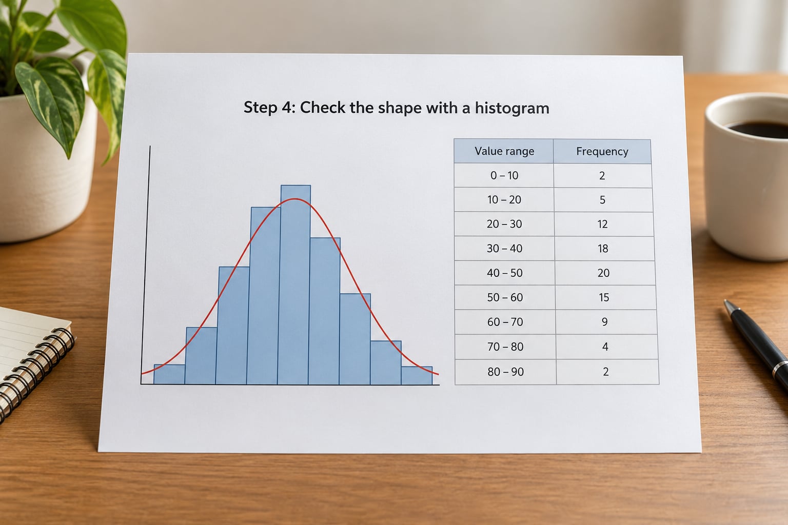
Look for three things: one peak in the middle, roughly equal spread on both sides, and no lone bar separated from the rest. A small skewness with a long spike at one end usually means a single outlier, and a kurtosis near zero with a flat rectangular shape usually means your data are grouped or rounded rather than genuinely normal. Also tick Boxplots with means for a quick read on spread and outliers, which is cheaper to interpret than the histogram.
Step 5: Use a normality test as supporting evidence
The Shapiro-Wilk test and the Kolmogorov-Smirnov test are in the same Statistics dialog box. Tick both, plus Normality tests, and SPSS adds a second table with a Sig. column for each. A Sig. value above .05 is conventionally read as no evidence against normality; below .05 is read as a deviation.
Here is the catch that confuses most users: with large samples, these tests detect trivial departures. At 2,000 cases, a skewness of 0.4 will produce a significant result, and that is not a problem worth fixing. At 20 cases, an obviously skewed distribution can still return Sig. above .05. With very small samples SPSS sometimes cannot compute the test at all and prints a note instead of a value.
If you find yourself staring at a Frequencies table where the shape statistics look fine but Shapiro-Wilk says Sig. = .001, you are not looking at a contradiction. The test is telling you the sample is large enough to detect a departure too small to matter for your analysis. Report both and explain, or move on without treating the test as the decision.
Step 6: Record and act on the results
Write down the skewness, the kurtosis, the standard error of each, the sample size and your decision, so the next person does not have to rerun anything. In APA 7 style, a sentence like this covers it:
The distribution of monthly income was moderately positively skewed (skewness = 1.42, SE = 0.11) and leptokurtic (excess kurtosis = 3.86, SE = 0.22), n = 284.
When the values are extreme, you have three options in order of preference. Transform the data first: a log or log10 transformation pulls in right-skewed positive data, a square root transformation works when values are counts or variances, and a Box-Cox transformation finds the best power for you automatically. Then consider winsorizing, which caps the extreme values at a set percentile instead of deleting them. Only after that, switch to a non-parametric test such as Mann-Whitney instead of an independent t-test, Wilcoxon signed-rank instead of a paired t-test, Kruskal-Wallis instead of one-way ANOVA, and Spearman instead of Pearson correlation.
Deleting outliers purely to tidy the shape is the option to use most carefully. Justify any removal in advance and report what you removed, or a reviewer will rightly ask whether you dropped inconvenient points.
Common Mistakes
Expecting kurtosis of 3 in the output. SPSS, R, pandas and Excel report excess kurtosis, where normal equals 0. If your reference book says 3, subtract 3 from what the software shows before comparing.
Judging normality on skewness alone. A symmetric distribution can have heavy tails, and a strong skew can sit on top of a perfectly normal-shaped peak if you ignore the extremes. Check both, every time.
Ignoring the Std. Error columns. A skewness of 0.6 with a standard error of 0.05 is a clear departure. The same 0.6 with a standard error of 0.35 is noise. Divide one by the other and the ambiguity disappears.
Relying on a single cutoff. Between -2 and 2 is a starting point, not a law. Sample size, discipline and the planned analysis all shift what counts as acceptable.
Treating a significant normality test as a verdict. Large samples make small departures significant. The test tells you a departure exists, not that your analysis is invalid.
Running the test on categorical codes. Skewness of a nominal variable has no interpretation. Frequencies and percentages are the right summary there.
Comparing values across two SPSS procedures. Frequencies and Descriptives handle missing data and weighting differently, so identical data can give values that differ in the second decimal. Check the sample size row in both tables before worrying.
Frequently Asked Questions
What are acceptable skewness and kurtosis values?
Most researchers treat skewness between -1 and 1 and excess kurtosis between -2 and 2 as acceptable for parametric tests. For structural equation modelling the limits are usually loosened to -3 and 3 for skewness and -10 and 10 for kurtosis. A better rule divides skewness by its standard error: a ratio under 2 is comfortable, over 3 is severe. Sample size matters more than the cutoff itself.
Should I use both skewness and kurtosis?
Yes, always report both. They describe different features: skewness covers asymmetry and kurtosis covers tail weight and peakedness. A distribution can be perfectly symmetric and still have heavy tails, which skewness alone would rate as fine. One short sentence covering both, with their standard errors and your sample size, is enough for most journals.
How do I find skewness and kurtosis in SPSS?
Go to Analyze, then Descriptive Statistics, then Frequencies. Move your variable into the Variable(s) box, click Statistics, and tick Skewness, Kurtosis and Std. Error. Click Continue then OK. The two values appear at the right-hand end of the Frequencies table with their standard errors beside them. Tick Charts and Histogram in the same dialog if you also want to see the shape.
Is a normality test required after checking skewness and kurtosis?
It helps, but it is not required. Shapiro-Wilk and Kolmogorov-Smirnov appear in the same SPSS Statistics dialog box and give a significance value in a second table. With large samples they flag tiny departures, and with tiny samples they miss real ones, so treat a significant result as information rather than a verdict. Report the shape values with their standard errors and note the test result if you ran it.
What should I do if my data are not normally distributed?
Transform first: log for right-skewed positive values, square root for counts and variances, Box-Cox when you want the software to choose the power. If that is not appropriate, winsorize the extremes or switch to a non-parametric test such as Mann-Whitney, Kruskal-Wallis or Spearman correlation. Check residuals rather than raw values when you are running regression, because it is the residuals that need to be normal.
Can skewness or kurtosis be fixed by deleting outliers?
Deleting cases will pull both values toward zero, but it changes what your data represent, not just how tidy it looks. If a case is genuinely outside the study population, remove it and say so. If it is a real observation that happens to be extreme, winsorize it or transform the variable instead, and report exactly what you did. Silent deletion is the option reviewers catch.
Conclusion
Start by confirming your variable is continuous and numeric, then run Frequencies in SPSS with Skewness, Kurtosis and Std. Error ticked. Read the values against the bands above, confirm the shape with a histogram, and use the skewness-to-standard-error ratio rather than a fixed cutoff. Then transform, winsorize or switch to a non-parametric test if the values demand it, and write the whole thing down in your results section.
Last reviewed for accuracy in 2026.