How to Split a Continuous Variable into Groups: Easy Guide 2026

Splitting a continuous variable into groups means creating a new categorical or ordinal variable from boundary values you choose. There are four ways to do it: equal-width ranges, equal-count quantiles, a median split, or cut points taken from domain knowledge. The original numeric variable stays in your data untouched.

The method matters more than the syntax. A colleague asking for “groups” usually wants one specific kind, and picking the wrong one gives you tables that will not answer their question. Most of the confusion on this topic is really confusion between equal-width and equal-frequency bins, so that is where this guide spends its time.

Table of Contents

1. 1What You Need
2. 2Step-by-Step: How to Split a Continuous Variable into Groups
3. 3How to Choose the Group Boundaries
4. 4How to Check the Distribution Before Splitting
5. 5How to Split the Variable in SPSS
6. 6How to Split the Variable in R
7. 7How to Split the Variable in Python
8. 8How to Split the Variable in Stata
9. 9How to Verify and Use the New Variable
10. 10Five Errors That Ruin a Split
11. 11Which Method Should You Use?
12. 12Syntax Cheat Sheet Across SPSS, Stata, R, and Python
13. 13Common Mistakes and Tips
14. 14Frequently Asked Questions
15. 15How do I split a continuous variable at the median?
16. 16Is it better to use equal-width groups or equal-frequency groups?
17. 17How many groups should I create from a continuous variable?
18. 18Should I analyze the grouped variable or keep using the continuous variable?
19. 19Why are my groups empty or unequal after splitting?
20. 20Can I split a continuous variable in Excel, SPSS, R, or Stata?
21. 21Conclusion

What You Need

A continuous variable is any numeric measure that can take any value in a range: age in years, income in dollars, reaction time in milliseconds, a test score from 0 to 100. Splitting it produces a categorical variable whose categories are ranges of the original, which makes it an ordinal variable because the categories still have a natural order.

That definition rules out the most common source of wasted afternoon: if your variable is already a set of categories, there is nothing to split. Recode it, or rename it. Grouping a categorical variable by its own levels is a different task.

Before you touch any software, get four things straight:

• The raw data file, open in the tool you actually use. Back it up first, because the most common damage is overwriting the continuous variable with the grouped one.
• A written statement of the grouping rule — the exact cut points, in numbers, before you implement them. “High and low scores” is not a rule. “Below 30, 30 to 59, 60 and above” is.
• The reason for the split: a t-test needs two groups, a one-way ANOVA needs three or more, a journal table might just need readability.
• A frequency table of the original variable, to check the range, the minimum, the maximum, and how many missing values you have.

Equal-width ranges use cut points at even numeric intervals — 0–29, 30–59, 60–89. Equal-frequency groups put roughly the same number of observations in each bin, so the boundaries land wherever the data happens to bunch up. Neither is right in general; which one you want depends on whether the numbers or the counts matter.

Step-by-Step: How to Split a Continuous Variable into Groups

How to Choose the Group Boundaries

Choose theory-based cut points when an external standard already defines the bands, equal-width ranges when the intervals have an intuitive size, and quantiles when every group needs comparable statistical weight. Start from your analysis goal and the shape of the data, not from a function name.

Suppose the variable is annual income in whole dollars, ranging from 0 to 150000, and you need four groups for a one-way ANOVA. Round-number cut points at 30000, 60000 and 90000 are defensible because anyone reading the table can interpret them without a key. That readability is the whole argument for domain cut points.

Quantiles are the better choice when your groups become the levels of an independent variable and you worry that a lopsided group leaves you with almost no observations in one cell. A right-skewed income distribution split at round numbers puts very few cases in the top band; quartiles fix that by construction.

The thing to avoid is choosing cutoffs after seeing which ones produce a tidy significant result. That is a fishing expedition dressed up as a method, and it will not survive review.

How to Check the Distribution Before Splitting

Look at the histogram first, then at skewness, then at the extremes. Equal-width ranges fit a roughly symmetric distribution well and fall apart on a badly skewed one, where a single high tail produces an almost empty final group.

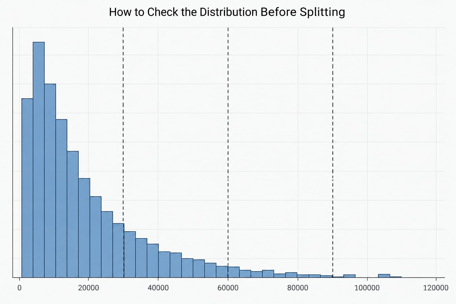
Ties and duplicates deserve attention before you pick boundaries. If a variable has few unique values — say a 1–7 rating scale — equal-frequency grouping into quartiles cannot work cleanly, because one value may need to sit in two bins or the bins collapse to fewer than you asked for. That is the source of the “why is my group empty?” question that comes up constantly on statistics forums.

Count missing values too. Decide up front whether they will be system-missing, excluded from the frequency table, or given their own category, and write that down with the cut points.

How to Split the Variable in SPSS

In SPSS use Transform > Recode into Different Variables to keep the original intact, or Transform > Visual Binning when you would rather drag break points on a histogram. Recoding into a different variable is the safer default because it never overwrites anything.

RECODE income (0 = "0 to 29999") (1 = "30000 to 59999")
        (2 = "60000 to 89999") (3 = "90000 and above")
        (SYSMIS = "Missing") INTO income_group.
VARIABLE LABELS income_group "Annual income group".
VALUE LABELS income_group 1 "Low" 2 "Lower middle" 3 "Upper middle" 4 "High".
VARIABLE LEVEL income_group (ORDINAL).
EXECUTE.

Note the key codes (1, 2, 3, 4) inside the quotes. Recode maps values, so the new variable holds those keys, and VALUE LABELS is what puts readable text on them. Use low-then-high codes so the variable sorts sensibly in every later table.

Visual Binning is faster when you have not decided the cut points yet: it draws the histogram, lets you drag the boundaries, and can write an equal-width or equal-count split in one click. Choose “Recode into different variables” when it writes the output so your code is documented.

How to Split the Variable in R

Base R’s cut() takes explicit break values. Pass right = FALSE so the intervals read as 0–29999, 30000–59999, with no double counting at the boundary.

income_group <- cut(income,
                   breaks = c(0, 30000, 60000, 90000, Inf),
                   right = FALSE,
                   labels = c("0 to 29999", "30000 to 59999",
                              "60000 to 89999", "90000 and above"))
table(income_group, useNA = "ifany")

Without right = FALSE, cut() uses right-closed intervals, so 30000 falls into the second group, not the first. That default is the origin of most off-by-one complaints. Inf as the last break keeps the largest values inside a group rather than dropping them.

For equal-sized groups use ntile() from base R, which places roughly the same number of cases in each bin:

income_quartile <- ntile(income, 4)
table(income_quartile)

# tidyverse equivalent
library(dplyr)
df <- df %>% mutate(income_quartile = ntile(income, 4))
df <- df %>% mutate(income_band = cut(income, quantile(income, seq(0, 1, 0.25)),
                                      include.lowest = TRUE, labels = FALSE))

ntile() is fast but it can split one identical value across two categories, which matters when you have many ties. When clean separation matters, use quantile breaks with include.lowest = TRUE, or the split_var() function from the sjmisc package, which carries an inclusive argument for exactly the few-unique-values problem.

How to Split the Variable in Python

pandas has two functions and choosing between them is the whole question. pd.cut() bins equal-width intervals from break values you supply; pd.qcut() bins equal-frequency quartiles from the data itself.

import pandas as pd

df["income_band"] = pd.cut(df["income"],
                           bins=[0, 30000, 60000, 90000, float("inf")],
                           right=False,
                           labels=["0 to 29999", "30000 to 59999",
                                   "60000 to 89999", "90000 and above"])

df["income_quartile"] = pd.qcut(df["income"], 4, labels=False)

df["income_band"].value_counts(dropna=False).sort_index()
len(df["income_band"].cat.categories)

Check the category count as well as the counts. If len(...cat.categories) comes back lower than the number of bins you passed, you have empty groups caused by duplicated break values or a gap in the data.

How to Split the Variable in Stata

Stata’s recode handles fixed cut points and lets you write the labels directly. The bounds are inclusive, so state both ends of each interval to avoid gaps or overlaps at the boundary.

recode income (0/29999 = "0 to 29999") ///
             (30000/59999 = "30000 to 59999") ///
             (60000/89999 = "60000 to 89999") ///
             (90000/.) = "90000 and above" into income_group
tabulate income_group

xtile income_group = nq(4), replace
tabulate income_group

Use xtile for equal-frequency groups. It reports the cut values it chose, so you can paste those into your methods section, and it handles small samples with repeated values more gracefully than hand-rolled code.

How to Verify and Use the New Variable

Run a frequency table on the grouped variable before you do anything else with it. You want to confirm that every case landed in exactly one category, that no group is empty or tiny, and that missing values behaved as you intended.

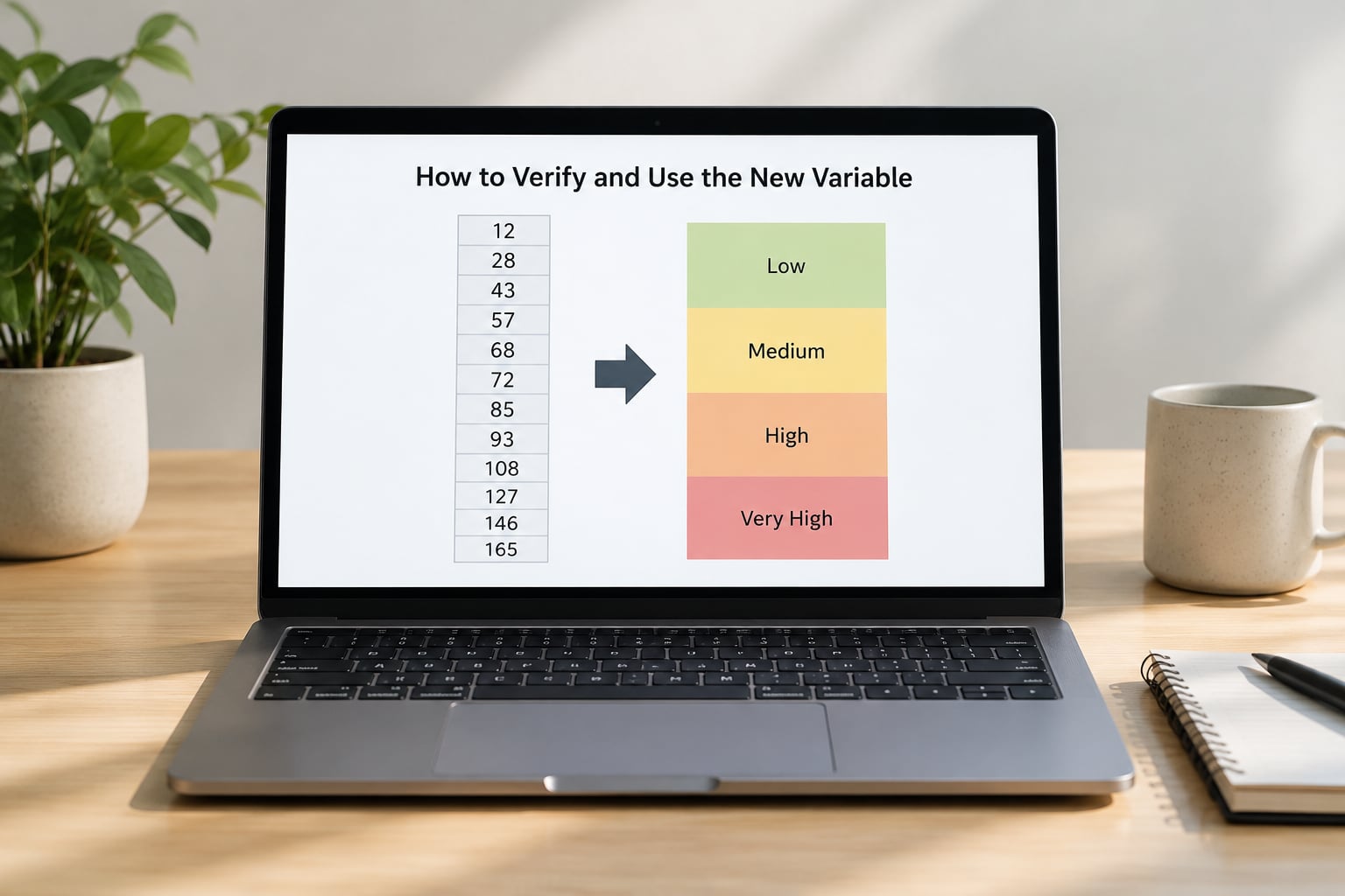
Then inspect the boundary cases. Sort the data by the original variable and look at the values sitting on each break point; if 30000 appears in both groups or in neither, your interval rule is off by one. Cross-tabulate the grouped variable against the original variable and you will spot it immediately.

Keep the original continuous measure in the dataset. Almost every downstream analysis — a correlation, a regression, a scatterplot — needs it, and deleting it is the step you cannot undo without rerunning the recode. If a reviewer asks why you grouped at all, having the continuous column makes the answer quick.

Five Errors That Ruin a Split

These are the mistakes that actually come up in practice, and each one has a simple fix.

1. Mixing up equal-width and equal-frequency. If you wanted groups of roughly the same size and used round-number cut points, you did not get what you asked for. Quantile-based breaks are the fix.
2. Off-by-one boundaries. Decide once whether the break value belongs to the lower or upper group, then write that rule down. In R, right = FALSE does it for you; in Stata, write both ends of every interval.
3. Unexplained group sizes. When the row count does not divide by the number of groups, the remainder has to go somewhere. Quantile functions handle it, but you should be able to say where it went.
4. Empty groups. Almost always caused by too few unique values or by hand-picked cut points landing in a gap where no observations sit.
5. Overwriting the original variable. Recode into a new name. In SPSS that means “Recode into Different Variables”; in R and Stata it means assigning to a fresh name rather than recycling the old one.

Which Method Should You Use?

Use equal-frequency groups when the group counts need to be comparable for statistical reasons, domain cut points when the bands must mean something to a reader outside your analysis, equal-width ranges when the variable is roughly symmetric and the intervals should be the same size, and a median split only when you specifically need two halves.

Method	What it makes equal	When to use it	Trade-off
Equal-width ranges	The size of each interval	Symmetric data, teaching examples, readable bands	Group counts can be wildly unequal
Equal-frequency quantiles	The number of observations per group	Skewed data, ANOVA or modelling where each group must carry weight	Boundaries land on odd numbers and shift between samples
Median split	Nothing, it simply halves the data	A quick high-versus-low comparison	Throws away everything except the ordering
Domain-defined cut points	Nothing, the rules come from outside the data	Official thresholds, policy bands, published categories	Needs a defensible source you can cite

Worth saying plainly before you go further: splitting a variable is not free. Any value inside a band is replaced by its category, so two people who scored 61 and 64 become the same case, and a t-test or ANOVA run on the grouped data throws away exactly the information you had. It also invites regression to the mean in any follow-up measurement, since the top group’s members were selected for a high first score and tend to fall back toward the middle. If your actual question is “do these two conditions differ”, analyse the continuous variable and let the model handle it. Group when a categorical input is genuinely required, or when the groups need to mean something to a reader.

Syntax Cheat Sheet Across SPSS, Stata, R, and Python

Task	SPSS	Stata	R	Python
Fixed cut points	Transform > Recode into Different Variables	recode … into	cut(x, breaks = )	pd.cut(x, bins = )
Equal-frequency groups	Transform > Visual Binning, equal counts	xtile, nq(4)	ntile(x, 4) or quantile breaks	pd.qcut(x, 4)
Median split	Recode below median as 1	egen med = median(x)	cut(x, 2) or quantile breaks	pd.qcut(x, 2)
Label the categories	VALUE LABELS	label define and label values	labels argument, or levels()	labels argument
Check group sizes	Frequencies > Charts > Frequencies	tabulate	table()	value_counts()

Common Mistakes and Tips

Almost every problem with a grouped variable traces back to a rule that was never written down. Fix that first and most of the list below disappears on its own.

• Write the cut points as numbers in your methods section. One sentence — “income was grouped into four bands using cut points of 30000, 60000 and 90000” — saves an email thread later.
• Report the resulting counts. A grouped results table without an N per category is not interpretable, because readers cannot tell a genuinely small group from one that lost cases to a boundary error.
• Name the categories so they sort correctly. Low-to-high key codes, or an ordered factor, prevents “High” landing before “Low” in a sorted frequency table.
• Keep the original continuous variable. Always. It costs one column and saves a rerun.
• Check for tiny groups before modelling. A band with four cases will produce an unstable estimate no matter which test you run.
• Justify the cut points, not just the method. Say where the numbers came from: a published standard, prior work, or the data quantiles. If the answer is “they looked about right”, that is the weak link a reviewer will pull.
• Do the split before you look at outcomes. Grouping after seeing the results is how analysis decisions quietly become outcome-driven.

Frequently Asked Questions

Conclusion

To split a continuous variable into groups, define your cut points, create a new categorical variable from them, label the categories, and check the frequency table before you analyse anything. The four routes are equal-width ranges, equal-frequency quantiles, a median split, and domain-defined thresholds, and the choice between equal-width and equal-frequency is the one most people get wrong.

Start by looking at the distribution and writing down why you chose those boundaries. Keep the original continuous variable in your data, and be honest in your write-up about what grouping costs. If nothing in your analysis truly needs a categorical input, the grouped variable belongs in a descriptive table, not in your inferential test.