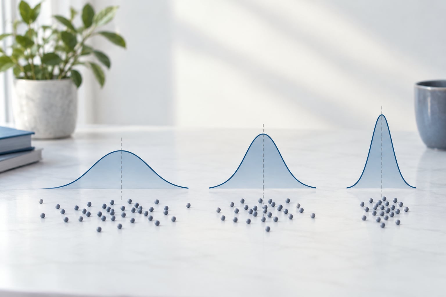
The central limit theorem says that, under suitable conditions, the distribution of a sample mean or proportion becomes approximately normal as the number of observations grows. It applies to the sampling distribution, not automatically to your raw data, and that single fact is what licenses most standard errors, confidence intervals and parametric tests you will ever run.
Here is the distinction that trips people up. When a lecturer or a forum thread tells you the CLT makes your non-normal data usable, what they mean is that the average of many independent observations behaves approximately like a bell curve. Your raw variable can stay stubbornly right-skewed, full of spikes and lumps, and the CLT still works. It never reshapes the data you collected. It reshapes the distribution of the statistic you compute from it.
Everything below builds on that point: what the theorem covers, what it does not, and how to check whether your own analysis qualifies.
Table of Contents
- 1What the central limit theorem means for your analysis
- 2How the central limit theorem works
- 3What conditions must be satisfied?
- 4Why sample size changes the analysis
- 5How the CLT affects standard errors and confidence intervals
- 6How the CLT is used in hypothesis tests
- 7What the central limit theorem means for your analysis in a t-test
- 8What changes for means, proportions, and other statistics
- 9How to check whether the approximation is trustworthy
- 10Common CLT mistakes and better alternatives
- 11Frequently Asked Questions
- 12Does the central limit theorem require my raw data to be normally distributed?
- 13Is a sample size of 30 enough for the central limit theorem?
- 14What should I do if my data contain extreme outliers?
- 15Does a large sample remove bias and make an analysis valid?
- 16How should I mention the central limit theorem in my research report?
- 17Conclusion: Start with what the CLT changes
What the central limit theorem means for your analysis
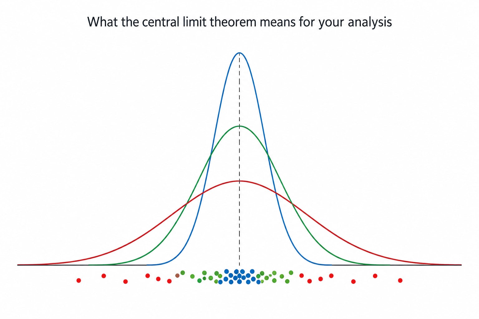
It means you can trust the arithmetic behind a p-value without trusting the shape of your data. Standard errors, t-distributions, confidence intervals and ANOVA all assume that the quantity you compute from many independent observations behaves approximately normally. The central limit theorem is the reason that assumption usually holds even when the underlying variable is nowhere near normal.
The theorem is about a sampling distribution, which is the distribution of a statistic across repeated samples. Draw a sample of 30, compute the mean, put it back, draw again, repeat a thousand times, and the thousand means form their own distribution. That distribution is what the theorem describes.
Your data’s distribution describes your people, your machines or your transactions. The sampling distribution describes what your statistic would have looked like across many possible studies. Mixing them up is the most persistent error in student and professional analyses alike, and it leads people to abandon valid t-tests simply because a histogram of raw values is lopsided.
How the central limit theorem works
Five terms carry most of the meaning. A population is every case you care about; a sample is the subset you actually observed. A parameter such as the population mean is fixed and usually unknown; a statistic such as the sample mean varies from sample to sample. The sampling distribution is the shape that varying statistic takes across repeated samples, and the standard error is the spread of that shape.
The theorem states that if the observations are independent and identically distributed with a finite mean and a finite variance, then the standardized sample mean approaches the standard normal distribution as the sample size grows. Written out in plain text: the sample mean X-bar is approximately normal with mean mu and variance sigma-squared divided by n.
| Quantity | What it describes | Typical shape |
|---|---|---|
| Population distribution | Every case in the population | Whatever reality produces, often skewed |
| Distribution of one observation | A single person, machine or transaction | Same shape as the population |
| Sampling distribution of the mean | The sample mean across repeated samples | Approximately normal for large n |
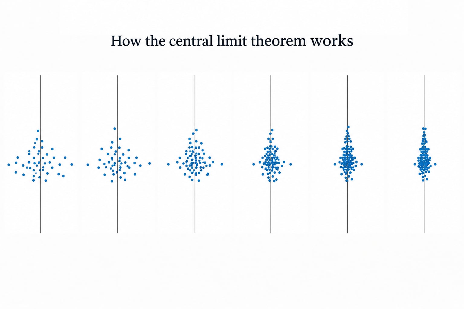
Take a quick worked case. Suppose the population of support tickets has a median wait of 8 minutes and a long upper tail. Draw samples of size 2, and the means swing wildly. At n = 10 they cluster nearer the population mean. By n = 50 the spread is visibly narrower and more symmetric, and the curve is close enough to normal that the ordinary standard error works well.
The spread shrinks by a factor of the square root of n. Going from n = 10 to n = 100 cuts the standard error in half; going from n = 100 to n = 400 cuts it by another half. That is the whole arithmetic behind “more data gives a tighter estimate”.
What conditions must be satisfied?
Four conditions decide whether the approximation is trustworthy, and each one is a check you can perform before you read a single p-value.
- Random or representative sampling. A convenience sample of volunteers or a survey that only reaches people with fast internet quietly breaks this condition. No sample size repairs a sample nobody chose at random.
- Independence of observations. Clustered sampling, repeated measures on the same subject, and panel data all create dependence. If one observation predicts the next, the average does not stabilise the way the theorem assumes.
- A quantitative or binary outcome. Means, proportions and rates are the natural cases. Categorical labels with no numeric ordering do not produce a sample mean.
- Finite variance and no extreme tail behaviour. Cauchy and Pareto style distributions have such heavy tails that the mean itself does not settle down no matter how large n grows.
A bounded population sampled without replacement is a milder issue. Once you sample a large share of the population, each remaining observation becomes slightly less likely to resemble the rest, which is why the common heuristic is to keep the sample below roughly ten percent of the population when that applies.
When you see strong skew, a small sample, dependence or extreme outliers, the honest response is to transform the outcome, resample, or switch to a method that does not lean on normality. Skewed continuous outcomes often behave well after a log or square-root transform. Discrete counts may need an exact method. Neither fix is a failure of the theorem; they are just a better model of your data.
Why sample size changes the analysis
Larger samples shrink random error and nothing else. That is the honest headline of the table below, and it is why “just collect more data” is bad advice for a badly designed study.
| What changes with a larger n | What a larger n does not fix |
|---|---|
| Sampling variability around the population value | Selection bias from a non-random sample |
| The standard error, which falls as one over the square root of n | Measurement error in the instrument itself |
| Precision of confidence intervals | A missing confounder or an omitted variable |
| Sensitivity of the normal approximation | A model that is misspecified for the process |
| Power, at fixed effect size and alpha | Dependence among observations |
This matters because precision is not validity. A sample of ten thousand people drawn only from one job title, one campus or one clinic gives you a beautifully narrow confidence interval around a number that does not describe the population you care about.
The familiar rule of thumb is that n of 30 or more makes the approximation safe. That number is a rough guide for a roughly symmetric distribution, and it is a poor guide otherwise. A symmetric uniform distribution is already close to normal in its sample means at n of about five. A moderately skewed distribution typically needs something in the twenties or thirties. A strongly skewed one may need far more, and a heavy-tailed one will never be rescued by sample size alone, because its variance is effectively infinite.
If your sample sits somewhere between ten and thirty, look at the shape of the distribution rather than the number. A histogram, a box plot, or a quick check of skewness will usually tell you more than any threshold rule.
How the CLT affects standard errors and confidence intervals
The standard error of the mean is sigma divided by the square root of n, and that single expression is the CLT’s most useful everyday output. When you see a confidence interval of plus or minus 1.96 standard errors around a mean, you are reading a normal approximation to the distribution of that mean, not a normal approximation to your data.
For a proportion the same logic applies, with the standard error written as the square root of p times one minus p divided by n. Because the variance shrinks as n rises, confidence intervals narrow, and a narrow interval is a statement about precision alone. It does not tell you the estimate is unbiased, that your sampling frame was representative, or that the relationship you measured is causal.
Wider intervals often point at a real problem worth investigating: a small sample, high variability, clustered sampling, or an outcome whose distribution has tails the normal curve cannot describe.
How the CLT is used in hypothesis tests
Every standard test you run is a rule for turning a raw difference into a standardised statistic and reading it against a reference distribution. The theorem supplies that reference distribution whenever the statistic is a mean or a proportion built from independent observations.
What the central limit theorem means for your analysis in a t-test
In an independent-samples t-test, the null hypothesis is that the two population means are equal. The test computes the difference in sample means and divides it by a pooled standard error, producing a t statistic that is compared against a t-distribution with a certain number of degrees of freedom.
Worked example. Group A has 40 observations with a mean of 62 and a standard deviation of 15. Group B has 40 with a mean of 70 and a standard deviation of 12. The difference is minus 8. The pooled standard deviation is close to 13.6, and the standard error of the difference is 13.6 divided by the square root of 80, which is about 1.52. The t statistic is therefore about minus 5.26 with 78 degrees of freedom, giving a p-value far below 0.001.
Now suppose the raw wait times behind those two groups are heavily right-skewed. The CLT says the distribution of the difference in means across repeated samples is approximately normal at this sample size, so the t-test is defensible. The skewness of the individual wait times does not invalidate it. That is the practical payoff of the theorem, and it is exactly what people doubt when they see a histogram.
The CLT does the same work for z-tests when the population standard deviation is known, for ANOVA across several groups, and for the significance tests on regression coefficients, where each coefficient is an average of many residual contributions.
One point deserves emphasis because it is routinely misunderstood. A p-value is the probability of observing data at least this extreme if the null hypothesis were true. It is not the probability that the null hypothesis is true, and it is not the probability that your result occurred by chance.
What changes for means, proportions, and other statistics
The theorem is a statement about averages. Extend your analysis past the mean and the support changes, sometimes quickly.
| Statistic | Normal approximation | When to use something else |
|---|---|---|
| Sample mean of a continuous variable | Reliable for moderate n even with skew | Very small n with strong skew or outliers |
| Sample proportion | Good when n times p and n times one minus p are both well above 10 | Small n or rare events, where an exact binomial is cleaner |
| Median | Weak; convergence is much slower than for the mean | Bootstrap or a rank-based test |
| Odds ratio or risk ratio | Usual only under large-sample or large-cell conditions | Small samples or sparse cells; exact or penalised methods |
| Correlation coefficient | Approximate via a transformation such as Fisher’s z | Few observations, or a non-monotone relationship |
| Heavy-tailed continuous outcome | Not supported | Median-based methods or a distribution-free estimator |
Proportions carry one more wrinkle worth remembering. When you approximate a discrete binomial count with a smooth normal curve, adding a continuity correction of half a unit substantially improves accuracy in small samples.
How to check whether the approximation is trustworthy
Run these checks before you trust the output, rather than after a reviewer questions it.
- Plot the raw data. A histogram or box plot by group reveals skew, gaps and isolated outliers that a summary table hides.
- Look at residuals in a model. For regression and ANOVA, the distribution that matters is the residuals, not the original variable.
- Check the design against the independence assumption. Cluster sampling and repeated measures break it, and no diagnostic plot will tell you so.
- Compare standard errors. Where software allows it, compare model-based standard errors with heteroskedasticity-consistent ones. A large gap is a signal that the usual assumptions are doing too much work.
- Simulate or bootstrap. Resample under your observed design and check whether the statistic behaves the way the normal approximation predicts. This is more informative than a normality test on raw data.
A formal normality test on the raw variable is not a gate. With large samples it will flag trivial departures, and with small samples it has little power to detect the ones that matter. Treat it as one piece of a picture, never as a decision on its own.
Common CLT mistakes and better alternatives
Five beliefs come up repeatedly, and each one has a straightforward correction.
The CLT makes my data normal. It does not, and no sample size will. What approaches normality is the sampling distribution of the mean. Keep plotting your raw values, and if they are badly skewed, consider a transform before modelling rather than after.
Thirty observations is always enough. Adequacy depends on the shape of the source distribution and on the statistic. Use n of 30 as a starting point for symmetric data and as a floor for skewed data, then look at the actual shape.
A bigger sample makes a biased study valid. Precision improves, validity does not. With selection bias or a serious confounder, a large sample gives you a narrow interval around the wrong number.
The CLT saves me when my observations are dependent. It does not. Clustered and repeated-measures designs need mixed models, generalised estimating equations, or a cluster-robust variance estimator.
It applies to every statistic. It applies cleanly to means and proportions. Medians, odds ratios in small samples, and heavy-tailed summaries need a different route, often a bootstrap or an exact method.
Frequently Asked Questions
Does the central limit theorem require my raw data to be normally distributed?
No. The theorem says nothing about the shape of your raw data. It says the distribution of the sample mean becomes approximately normal as n grows, under independence, random sampling and finite variance. Your raw variable can be strongly right-skewed or full of lumps and the approximation for the mean can still be sound. What must be close to normal is the sampling distribution of the statistic, not the observations themselves.
Is a sample size of 30 enough for the central limit theorem?
Thirty is a rule of thumb rather than a threshold, and it is a rough guide only. It is reasonable for a roughly symmetric distribution and often optimistic for a strongly skewed one, which may need a substantially larger sample. Heavy-tailed distributions are not rescued by sample size at all because their variance is effectively infinite. Judge adequacy from the shape of your distribution and the statistic you are computing, not from the number alone.
What should I do if my data contain extreme outliers?
Start by plotting the data and checking whether the outliers are errors, legitimate rare cases, or a sign of a heavier tail than your model assumes. Correct genuine recording errors. For legitimate extremes, a log or square-root transform often restores symmetry. If the tail is genuinely heavy, switch to methods built for it, such as a bootstrap or a rank-based test. Simply collecting more observations will not fix a heavy tail.
Does a large sample remove bias and make an analysis valid?
No. A larger sample shrinks sampling variability, which narrows confidence intervals and raises power. It does not repair selection bias, a non-representative sampling frame, measurement error, an omitted confounder, or a misspecified model. The result is a precise estimate of the wrong quantity, which is why design matters more than sample size. In short, larger n buys precision, not validity.
How should I mention the central limit theorem in my research report?
State the conditions you relied on rather than naming the theorem alone. Write something like: independent observations obtained by random or representative sampling, an outcome with finite variance, and a sample size large enough for the observed skewness to give an adequate normal approximation. Add that a skewed outcome was transformed, or that a non-parametric alternative was used instead. That short sentence shows a reviewer you checked the assumptions.
Conclusion: Start with what the CLT changes
The central limit theorem changes one thing about your analysis: it makes an approximate normal reference distribution available for the mean, so standard errors, confidence intervals and t-based tests stay usable when your raw data is obviously not normal. It does not normalise your data, it does not repair bias, and it does not extend itself to every statistic.
Before you run the next test, work through four questions. Are the observations independent, or does the design involve clusters or repeated measures? Was the sample random or representative rather than convenient? What does the shape of the distribution look like, and are there extreme outliers? And which statistic am I actually testing, a mean, a proportion, or something less forgiving?
If the first three answers are clean and the statistic is a mean or a proportion, the approximation is almost certainly on your side. If any of them is not, choose a transform, a bootstrap, or a method built for the design you actually used.