Tukey vs Bonferroni Post Hoc Tests Explained for ANOVA (2026)

Both tests are post hoc follow-ups to a significant ANOVA, and this guide to tukey vs bonferroni post hoc tests explained for ANOVA covers where they split. Tukey’s HSD spends a single critical value across the whole family of pairwise comparisons; Bonferroni splits your alpha level into m smaller pieces.

The short version: use Tukey’s HSD when you have equal group sizes and equal variances and want every pairwise comparison. Use Bonferroni when you need a correction that assumes nothing about the shape of your data, or when you’re testing a small number of planned contrasts. Tukey keeps more power, Bonferroni is more conservative.

Below is the full comparison — the formulas, the assumptions, what each software command actually does, and a worked five-group example where the two methods disagree on one pair of means.

Table of Contents

1. 1Tukey vs Bonferroni Post Hoc Tests at a Glance
2. 2What Are Tukey and Bonferroni Post Hoc Tests?
3. 3How Tukey and Bonferroni Control Familywise Error
4. 4Tukey vs Bonferroni: Assumptions and Data Requirements
5. 5When to Use Tukey or Bonferroni After ANOVA
6. 6Use Tukey when groups are balanced and homoscedastic
7. 7Use Bonferroni when group sizes or variances are uneven
8. 8Use Bonferroni for a small number of planned contrasts
9. 9Use Bonferroni for repeated-measures and mixed designs
10. 10Consider Dunnett when you have one control group
11. 11Consider Scheffe, Games-Howell, or Dunn when assumptions break
12. 12How to Interpret the Results
13. 13How to read a Tukey vs Bonferroni output table
14. 14How to Run the Tests in SPSS, R, Stata, and SAS
15. 15SPSS, JASP and jamovi
16. 16R
17. 17Stata
18. 18SAS
19. 19Tukey vs Bonferroni Examples With Five Groups
20. 20Which Should You Choose?
21. 21Frequently Asked Questions
22. 22When not to use Bonferroni correction?
23. 23What is the Bonferroni test used for in post-hoc testing?
24. 24When should a Tukey post-hoc test be used?
25. 25Can you explain the Bonferroni correction in simple terms?
26. 26Can I use Tukey or Bonferroni with repeated-measures ANOVA?
27. 27How do I report Tukey and Bonferroni results in a paper?

Tukey vs Bonferroni Post Hoc Tests at a Glance

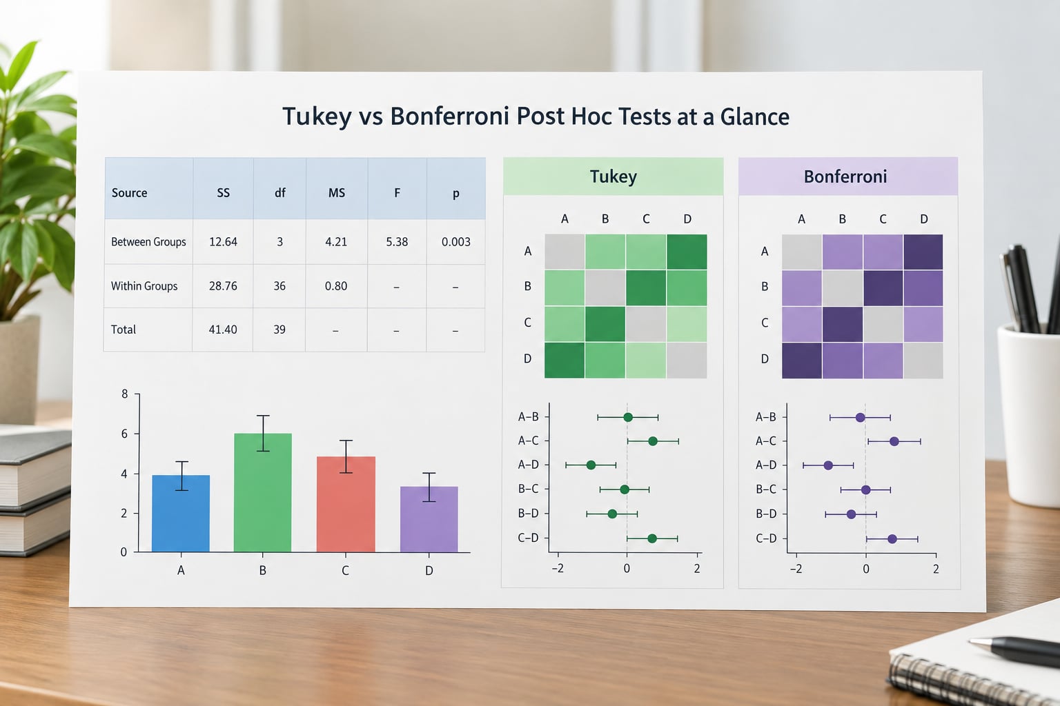
Criterion	Tukey’s HSD	Bonferroni
Primary purpose	Find every pair of group means that differs	Correct any set of m comparisons so the chance of one or more false positives stays at alpha
What it controls	Family-wise error rate (FWER), strongly	Family-wise error rate, valid under any dependence between tests
Threshold rule	One critical value q from the studentized range distribution, giving an honestly significant difference	alpha divided by m, or raw p multiplied by m
Key assumption	Homogeneity of variance; equal n for the basic HSD version	None beyond the omnibus test’s own assumptions
Statistical power	Higher for all-pairs comparisons of many groups	Lower; some real differences disappear after correction
Best fit	One-way ANOVA, equal n, equal variances, three or more groups	Unequal n, unequal variances, repeated measures, planned contrasts
R function	TukeyHSD()	pairwise.t.test(…, p.adjust.method = “bonferroni”)
SPSS menu	One-Way ANOVA > Post Hoc > Tukey	One-Way ANOVA > Post Hoc > Bonferroni

What Are Tukey and Bonferroni Post Hoc Tests?

A post hoc test is a follow-up analysis run after a significant omnibus test. The omnibus F-test in a one-way ANOVA has a single null hypothesis: all group means are equal. Reject it and you’ve learned that at least one pair differs, which is exactly the question most analyses don’t answer.

The reason you need a correction at all is that the omnibus test doesn’t tell you how many comparisons you’re about to make. With five groups you have ten pairs, and running ten independent t-tests at alpha = 0.05 gives you a family-wise error rate, FWER = 1 − (1 − 0.05)^m, of about 40 percent.

Comparisons (m)	Chance of at least one false positive at alpha = 0.05
1	5%
3	14%
6	26%
10	40%
20	64%

That’s the multiple comparisons problem in one line, and it’s why both Tukey and Bonferroni exist. They attack it differently. Bonferroni is a generic correction that can be bolted onto any set of p-values. Tukey is a single procedure designed specifically for pairwise group comparisons, and it knows your ANOVA already produced a pooled error term.

Both are usually conditional on the omnibus test reaching significance. Some methodologists prefer to drop that condition and report adjusted pairwise comparisons regardless, and either route is defensible if you say which one you used.

How Tukey and Bonferroni Control Familywise Error

Bonferroni controls FWER with pure arithmetic, and you can do it by hand on a napkin. With m comparisons and a chosen alpha of 0.05, each test runs at 0.05/m instead of 0.05. Equivalently, multiply each raw p-value by m and cap the result at 1.

So with five groups and ten comparisons, the Bonferroni threshold is 0.005. A pair whose raw p-value is 0.012 is no longer significant, and no amount of arguing changes that. It comes from Boole’s inequality, which means the correction is valid even when your comparisons share scores and are statistically dependent.

Tukey takes a different route. It computes a q statistic, which is a mean difference divided by the standard error of that difference, and compares it to a critical value drawn from the studentized range distribution. That critical value already accounts for the number of groups being compared, so you make every decision against one threshold instead of m of them.

The standard error underneath Tukey is built from the pooled within-group variance from the ANOVA itself, plus an adjustment for unequal group sizes when you use the Tukey-Kramer version. That’s the whole reason Tukey is more powerful here: the omnibus test has already estimated the error term for you, and Tukey reuses it instead of estimating a fresh one for every pair.

The practical consequence is that Bonferroni over-corrects when comparisons are correlated, which they usually are inside a single dataset. Tukey exploits that correlation, so it keeps more of the real differences that are sitting just past the threshold. With ten comparisons, Bonferroni may miss a genuine effect that Tukey catches.

Tukey vs Bonferroni: Assumptions and Data Requirements

Neither method is assumption-free, but the list of assumptions is much shorter for Bonferroni. Here’s what each one needs beyond the omnibus test’s own assumptions.

Requirement	Tukey’s HSD	Bonferroni
Normality of residuals	Needed for the studentized range distribution	Inherited from the omnibus test
Independent observations	Required	Required
Equal group sizes	Required for plain HSD; use Tukey-Kramer if not	Not required
Equal variances across groups	Required; check with Levene’s test	Not required for the correction itself
Repeated-measures or mixed design	Does not apply directly	Usable, and often the default choice

That last row is the one that catches people out. On AskStatistics, the repeated short answer is consistent: “Tukey’s doesn’t work with RM-ANOVA. Bonferroni is typically used.” That’s about the raw analysis, because a repeated-measures ANOVA has several error terms and a pooled within-group variance no single number can summarise.

Modern practice softens this a bit. You can fit a mixed model and run Tukey-adjusted contrasts on the estimated marginal means, which handles the design correctly. What you can’t do is paste repeated-measures data into a one-way ANOVA and trust the Tukey output.

For unequal variances with unequal sample sizes, Tukey’s adjustment isn’t enough on its own. Games-Howell is built for exactly that case, and Dunn’s test is the nonparametric follow-up to Kruskal-Wallis.

When to Use Tukey or Bonferroni After ANOVA

Match the method to your design, not to habit. These are the situations that come up most often in practice.

Use Tukey when groups are balanced and homoscedastic

Equal sample sizes, similar variances, three or more groups, and every pair genuinely matters to your question. This is the textbook case and the one where Tukey’s extra power is real rather than nominal. It’s also the cultural default in biology and life sciences, which is why you’ll see it recommended by default in a lot of lab methods sections.

Use Bonferroni when group sizes or variances are uneven

Unbalanced designs with unequal variances are where plain Tukey starts to stretch. Bonferroni makes no shape or balance assumption, so it’s the safer choice when you haven’t checked homogeneity of variance, or when a covariate adjustment has left the groups with different residual spreads.

Use Bonferroni for a small number of planned contrasts

If you planned two or three specific comparisons before collecting data and you don’t need every other pair, Bonferroni is often more appropriate than Tukey. Tukey spends its alpha on all possible pairs whether or not you care about them, so you’re paying for comparisons you never intended to make.

Use Bonferroni for repeated-measures and mixed designs

SPSS doesn’t offer Tukey as a post-hoc option in its repeated-measures ANOVA dialog at all, which is a good hint about the conventional wisdom. Bonferroni is built into that menu, and estimated marginal means with pairwise comparisons give you a defensible Tukey-adjusted alternative.

Consider Dunnett when you have one control group

If every comparison runs against a single control condition, Dunnett is more powerful than either method here because it only spends alpha on the comparisons you actually make.

Consider Scheffe, Games-Howell, or Dunn when assumptions break

Scheffe is the right pick when you need simultaneous inference for arbitrary contrasts, or when you plan to make claims about linear combinations beyond simple pairwise differences. Games-Howell covers unequal variances with unequal n. Dunn handles a nonparametric omnibus test.

How to Interpret the Results

Post-hoc output looks different in every package, so learn to read the columns rather than the layout. What you’re looking for is the adjusted p-value, the confidence interval, and the estimated difference between each pair of group means.

How to read a Tukey vs Bonferroni output table

In R, TukeyHSD() returns a named matrix with four columns: diff, lwr, upr and p adj. The intervals there are simultaneous, meaning the whole set of them covers 95 percent of the time at once rather than each one separately. pairwise.t.test() returns a lower-triangular matrix with p values and confidence intervals instead, which is why the two outputs never line up neatly in a table.

Look for adjusted p-values below your alpha, not raw ones. A raw p of 0.02 after a ten-comparison Bonferroni correction is really 0.20, and reporting it as 0.02 is the single most common error in this part of an analysis. Many software dialogs quietly report the adjusted value only, so check which one you’re reading before you write it down.

A significant omnibus test does not mean every pair differs. With three groups, there are only three pairs; with six, there are fifteen, and the correction grows with each one. It’s entirely normal to get an overall F-test with p < .001 and then see just two significant pairs. That combination is a real result, not a bug.

The flip side is the question that comes up constantly on AskStatistics: a significant interaction that produces nothing significant under Tukey. That usually reflects power rather than an error. Pairwise tests on an interaction are conservative because each cell mean is estimated with more variance than a marginal mean, and the marginal contrast is often the one worth reporting.

Report the mean difference with its interval and an effect size where possible. A pairwise difference of 4.2 points with a 95 percent interval of 0.3 to 8.1 tells a reader far more than a bare p-value ever will. Reviewers increasingly ask for Cohen’s d on each significant pair, and none of the built-in post-hoc dialogs compute it for you, so plan to add it after the fact in R with a short loop over the pairs or in JASP under Descriptive Statistics.

One more detail worth checking before you commit: whether the interval your software prints is simultaneous or pointwise. Tukey and Bonferroni both produce simultaneous intervals by default, which means the whole set together covers 95 percent of the time. Some software quietly switches to pointwise intervals when you ask for them at a different confidence level, and those are narrower and easier to cross zero.

How to Run the Tests in SPSS, R, Stata, and SAS

All four mainstream packages will do this work. The software applies the correction for you; it does not decide which method is scientifically right for your design, so that decision stays yours.

SPSS, JASP and jamovi

In SPSS, run Analyze > Compare Means > One-Way ANOVA, then open the Post Hoc button and tick Tukey and Bonferroni separately to see both tables. SPSS’s Bonferroni entry is plain Bonferroni, not Holm. JASP follows the same logic under ANOVA > Post Hoc Tests, and jamovi puts it in ANOVA > Post Hoc.

R

Two functions, two shapes:

data(PlantGrowth)
fit <- aov(weight ~ group, data = PlantGrowth)
TukeyHSD(fit)

pairwise.t.test(PlantGrowth$weight, PlantGrowth$group,
                p.adjust.method = "bonferroni")

Watch the default. p.adjust() defaults to Holm, not Bonferroni, and pairwise.t.test() inherits that default. If a methods section says Bonferroni, name the method explicitly rather than relying on what the function does out of the box.

For a model with covariates or repeated factors, use estimated marginal means instead:

library(emmeans)
m <- aov(weight ~ group, data = PlantGrowth)
emmeans(m, ~ group) |> pairwise.emmeans(adjust = "tukey")

Stata

Fit the model, then ask for adjusted contrasts:

regress weight i.group
margins group, pwcompare(tukey)
margins group, pwcompare(bonferroni)

SAS

The ADJUST= option sits on the LSMEANS or MEANS statement:

proc glm data=work.plantgrowth;
  class group;
  model weight = group;
  lsmeans group / adjust=tukey diff cl;
  lsmeans group / adjust=bonferroni diff cl;
run;

In PROC MIXED, the same option is spelled diff adjust=tukey cl= on the lsmeans statement. Either way, requesting both in one run is a cheap way to see whether the choice changes any of your conclusions before you commit to one in the write-up.

Tukey vs Bonferroni Examples With Five Groups

Five treatment groups with 20 observations each gives 95 error degrees of freedom and a pooled within-group variance of 100, so the standard error of any single pairwise difference is sqrt(2 × 100 / 20) = 3.16. The group means are 30.0, 25.8, 20.4, 16.9 and 19.6.

The omnibus test comes first: between-groups sum of squares is 2,226 on 4 degrees of freedom, giving F = 5.57 with p < .001. Ten comparisons are now permitted, and here’s where the two methods part company.

Pair	Mean difference	Raw p	Bonferroni (p × 10, threshold 0.005)	Tukey (critical difference 8.8)
A vs B	4.2	0.187	No	No
A vs C	9.6	0.003	Yes	Yes
A vs D	13.1	< .001	Yes	Yes
A vs E	10.4	0.0015	Yes	Yes
B vs C	5.4	0.090	No	No
B vs D	8.9	0.006	No	Yes
B vs E	6.2	0.053	No	No
C vs D	3.5	0.269	No	No
C vs E	0.8	0.803	No	No
D vs E	2.7	0.398	No	No

Bonferroni calls three pairs significant. Tukey calls four, because its critical difference of about 8.8 catches B versus D at 8.9 while the Bonferroni threshold of 0.005 rejects it at 0.006. Holm also finds four here, which is its usual behaviour: it matches or beats plain Bonferroni and often lands near Tukey.

That one extra pair is the whole argument in miniature. Tukey and Holm spend their alpha more efficiently on correlated comparisons, so they retain differences that plain Bonferroni throws away. The trade is that Tukey needed equal variances to earn that power, and if that assumption doesn’t hold, the conservative version is the honest one.

Which Should You Choose?

Tukey’s HSD for standard all-pairs comparisons after a balanced one-way ANOVA with equal variances. Bonferroni when you need a correction that makes no distributional assumptions, when group sizes are uneven, when you’re in a repeated-measures design, or when a reviewer has asked for it by name. For anything else, reach past both of them: Dunnett against a single control, Games-Howell for unequal variances with unequal n, Scheffe for arbitrary contrasts, Dunn after Kruskal-Wallis.

A usable methods sentence, with the numbers filled in from the Bonferroni column above:

Bonferroni-adjusted pairwise comparisons indicated significant differences between Groups A and C (mean difference = 9.6, 95 percent CI [3.3, 15.9], adjusted p = .03), A and D (13.1, CI [6.8, 19.4], adjusted p < .001) and A and E (10.4, CI [4.1, 16.7], adjusted p = .015). All other pairwise comparisons were not significant after correction.

Five mistakes show up again and again. Adjusting an already-adjusted p-value a second time is the first; if software produced the adjusted value, leave it alone. The second is reporting raw p-values from a corrected analysis. The third is running parametric post-hoc tests after a nonparametric omnibus test such as Kruskal-Wallis, where the answer is Dunn’s test with a correction. The fourth is ignoring the interaction and running a single set of post-hoc comparisons on every cell of a factorial design. The fifth is treating a null post-hoc result as evidence of no effect, when it may just mean the study had too little power for that particular pair.

This page is educational. If a correction choice genuinely changes a conclusion in your own study, talk it through with a statistician or your supervisor before you write it up.

Frequently Asked Questions

Start by running the omnibus test and confirming your assumptions, especially Levene’s test for equal variances and whether group sizes are balanced. Then pick Tukey if that check passes and you want every pair, pick Bonferroni if it doesn’t or if the design is repeated-measures, and run both once so you know whether the choice changes any conclusion before you write it up. If you only remember one thing from this comparison, remember that a correct adjustment you can defend beats a powerful one your reviewer rejects.