How to Run a Mixed ANOVA With Between and Within Factors 2026

To run a mixed ANOVA with between and within factors, you enter every repeated measure as its own column, then open Analyze > General Linear Model > Repeated Measures in SPSS, move your grouping variable into the Between Subjects box, and read the within- and between-subjects tables separately. With one between factor and one within factor you get three results: a main effect of the between factor, a main effect of the within factor, and an interaction.

This is the analysis behind almost every pre/post treatment-versus-control dissertation chapter. The awkward part is rarely the click path. It is deciding which of your variables is within-subjects and which is between-subjects, and then getting the data into the shape the dialog expects.

Below I walk through the whole process: the design, the data layout, the assumption checks, the exact SPSS dialog, reproducible R code, how to read the output, and an APA template you can paste into your results section.

Table of Contents

1. 1What You Need
2. 2How to decide: within or between?
3. 3Software and versions
4. 4Data layout: one row per participant
5. 5Step-by-Step
6. 6How to Run a Mixed ANOVA With Between and Within Factors
7. 71. Define Your Factors and Hypotheses
8. 82. Prepare and Check the Data
9. 93. Check the Mixed ANOVA Assumptions
10. 104. Run the Analysis in SPSS
11. 115. Run and Verify the Analysis in R
12. 126. Interpret the Main Effects and Interaction
13. 13Tests of Within-Subjects Effects
14. 14Tests of Between-Subjects Effects
15. 15What those numbers mean
16. 16Unpacking the interaction
17. 177. Report the Results and Save the Output
18. 18Common Mistakes
19. 19Frequently Asked Questions
20. 20What if my mixed ANOVA design is unbalanced or has unequal group sizes?
21. 21How many within-subject factors can I include in one mixed ANOVA?
22. 22What should I do when Mauchly’s test indicates that sphericity is violated?
23. 23Can I use a mixed ANOVA when my within-subject factor has only two levels?
24. 24Why do my SPSS and R results use different error terms or degrees of freedom?
25. 25What information must I include when reporting a mixed ANOVA in an academic paper?
26. 26Conclusion

What You Need

A mixed ANOVA needs at least two independent variables, and they have to be of different types. Every factor is either within-subjects or between-subjects, and the two types answer different questions.

• Between-subjects factor: each participant belongs to exactly one level, and different participants sit in different levels. Treatment versus control is the classic example. The variable is usually a single column of group labels.
• Within-subjects factor: every participant is measured on every level, so the measurement is repeated on the same person. Time points, body sites, devices or task types are typical. Each level lives in its own column.
• Dependent variable: the numeric score you are comparing, one column per within-subjects level.

Only the between factor gets its own column. The within factor is spread across several score columns, which is why people get stuck.

How to decide: within or between?

Ask one question: did every participant experience every level of this variable? If yes, it is within-subjects. If participants were split into separate groups, it is between-subjects.

Research scenario	Variable	Correct type	Why
Treatment vs control, measured at pre-test and post-test	Group	Between	Nobody is in both arms of the trial
Same treatment vs control study	Time point	Within	Every participant is measured at both points
Blood pressure recorded on each arm in turn	Side	Within	Each person has both sides measured
Pressure pain threshold across 10 body sites	Site	Within	One person supplies all 10 readings
Clinicians vs patients in a usability study	Participant type	Between	Each person is only one type
Usability task run on phone, tablet and laptop	Device	Within	Everyone tries all three devices
Learning method A vs method B across three tests	Method and test number	Between and within	One splits the people, one repeats on them

The side-and-site case is the one that trips people up most. A shoulder pain study with pressure pain thresholds at multiple sites on both sides is a 2 by 10 within-subjects design, and the treatment arm adds a third, between-subjects factor. Nothing in the variable name tells you the type. Only the design does.

Software and versions

IBM SPSS Statistics desktop is the most common route, and the paths below are for releases 25 through 29. Newer builds occasionally rename a checkbox, but the dialog sequence has been stable for years. In R, the afex package handles repeated measures cleanly. Python users usually reach for pingouin. Stata users run mixed with the rtt option, which adds the repeated-measures table to the output.

Also useful: a mixed-effects model in R, Stata or MATLAB Central’s own discussions come up constantly, and a linear mixed-effects model is the right upgrade when your groups are unbalanced. I cover that decision near the end.

Data layout: one row per participant

SPSS needs wide format. Each row is one participant, the group label sits in one column, and every within-subjects level gets a separate score column. Here is the shape for a Group (between, 2 levels) by Time (within, 3 levels) study with 24 participants.

id	group	pre	mid	post
101	Intervention	52	57	63
102	Intervention	55	60	66
103	Control	54	55	57

That is the whole layout. If your data arrived long (one row per participant per time point, with a time label column), you have to reshape it before SPSS will accept it.

Step-by-Step

How to Run a Mixed ANOVA With Between and Within Factors

A mixed ANOVA is an independent-samples comparison and a repeated-measures comparison running in the same model. The model splits total variability into a between-subjects part (differences among people) and a within-subjects part (differences across repeated levels inside each person), then tests each effect against its own error term.

That is why the output is split. Within-subjects effects — the within factor and the interaction — are tested against the error term called subjects by time. The between-subjects main effect is tested against the error term that captures person-to-person variation. Reading the wrong table is the most common reporting mistake in mixed designs.

The example running through this article is a 2 by 3 mixed design. Group (intervention, control) is between-subjects; time (pre, mid, post) is within-subjects; the dependent variable is a wellbeing score. Group means run 52.4, 58.1 and 63.7 across the three points, while control means run 53.8, 55.2 and 56.9. The lines diverge, which is exactly what the interaction is designed to catch.

1. Define Your Factors and Hypotheses

Write the design down before you touch the data. For each variable, record its role and whether it is within or between.

In the worked example:

• Between-subjects factor: group, two levels (Intervention, Control), 12 participants per level.
• Within-subjects factor: time, three levels (pre, mid, post), measured on everyone.
• Dependent variable: wellbeing score, same scale at each time point.

Then state three hypotheses. H1, main effect of time: mean wellbeing scores are equal at pre, mid and post. H2, main effect of group: intervention and control participants have equal mean scores overall. H3, interaction: the change in score over time is the same in both groups.

H3 is the one your research question usually depends on. In an intervention study the interesting claim is almost never “scores went up” — it is “scores went up more in the treated group.” That is the interaction, and it is also the effect you must interpret first when it is significant.

2. Prepare and Check the Data

Four things go wrong at this stage, so check all four before running anything.

1. One row per participant. Count your rows and compare against your participant count. More rows than people means long format.
2. Unique participant IDs. The ID column must have no duplicates and no blanks. SPSS treats the repeated-measures factor as nested inside this variable, so duplicates silently corrupt the error term.
3. Clean factor labels. No stray spaces (“Intervention ” and “Intervention”), no mixed case, no numeric codes you have forgotten. Recode through Transform > Recode into Different Variables.
4. Missing values declared. Set the missing-value cells explicitly in Variable View so SPSS excludes them rather than reading them as zero.

To convert long format to wide in SPSS, use Transform > Restructure Data > Restructure into Wide Cases. Put id and group in the Identifying Cases box, time in the Grouping Variable box, and the score in the Variable to Restructure box. Click the cell in the Name and Label grid that lines up group with time, and type a prefix such as score_.

In R the same job is one line:

wide <- reshape(long, idvar = "id", timevar = "time", direction = "wide")
# pre_mid_post become score_pre, score_mid, score_post

Once the layout is right, run Data > Sort Cases by id and check that every participant has a value in all three time columns. A participant missing the post-test is a listwise deletion, and SPSS will drop the entire participant from the model, not just the missing cell. With 10% attrition that can quietly shrink your sample by a third, so check the “Listwise” count in the output against the number you started with.

3. Check the Mixed ANOVA Assumptions

Four assumptions matter, and only one of them is specific to repeated measures.

Independence. Each participant contributes to one group only, and one group’s scores are independent of another’s. If the same people appear twice under two labels, your design is not between-subjects at this factor.

Normality of residuals. ANOVA tolerates moderate departures from normality when groups are balanced and around 12 or more per cell, but check anyway. Run Analyze > Descriptive Statistics > Explore, move the three score columns in, then click Plots and tick Normality plots with the Filled circles and Regression line option. A Shapiro-Wilk p above .05 is fine; below that, look at the dots rather than the test.

Homogeneity of variance between groups. Levene’s test appears automatically in the SPSS output. A p above .05 means group variances can be treated as equal. Below .05 means they are not, and the F test for group is no longer trustworthy as it stands.

Sphericity applies to every within-subjects effect with three or more levels, including the interaction. It assumes that the variances of all pairwise differences between levels are equal, which is a strong claim and often false. Mauchly’s test of sphericity in the output checks it. A p above .05 means sphericity holds and you report the uncorrected degrees of freedom. Below .05 means use the Greenhouse-Geisser correction.

Two things worth knowing. With only two within-subjects levels, sphericity holds automatically — there is no test to worry about, which is one reason the 2 by 2 mixed design is so common. And when you do need a correction, Greenhouse-Geisser epsilon below 0.75 is the conservative choice; epsilon of 0.75 or above means Huynh-Feldt is less severe. SPSS reports both, and you report the one you justify.

If Levene’s test comes back significant, you have three options in order of preference: check whether a skewed score variable is driving it and transform it (a square root or log often settles count and wellbeing scores), move to a linear mixed-effects model with group as a random slope, or accept the result and report it honestly as a limitation. Welch-type corrections for mixed designs are not built into the SPSS dialog, so a mixed model is usually the cleaner route.

4. Run the Analysis in SPSS

Go to Analyze > General Linear Model > Repeated Measures. This is the dialog for one or more between factors combined with one or more within factors measured across several columns. (Analyze > General Linear Model > Mixed is a different procedure, used when the repeated measure is a continuous covariate rather than discrete levels.)

1. Name the within factor. In the box at the top, type a name with no spaces — time. Set Number of Levels to 3. Click Add.
2. Check the Measure box. Tick the time cell under Measure to move it into the dependent measures list.
3. Move the score columns. Click the Time cell and drag pre, mid and post into the box underneath so each level has one variable.
4. Define. Click Define. SPSS maps each within level to its column; check the mapping before moving on.
5. Between Subjects. Click the Between Subjects button, type the between factor name in the Name box — group — set its number of levels, click Add, then drag the group column from the variable list into the box.
6. Options. Tick Descriptives, Estimates of effect size, Homogeneity tests, and Residuals (Residuals and Normality plots). These produce the descriptive table, Levene’s test, partial eta squared and the residual checks.
7. EM Means. Move group into the Dependent Variable area and, in the Displaying table box, tick Group for time and Time for group. This gives you the estimated marginal means you need for simple effects after a significant interaction.
8. Plots. Put time on the horizontal axis and group as separate lines to generate the profile plot.
9. Options in the right-hand panel. Leave the model at full factorial. Set the confidence interval to 95%.
10. OK.

If you have a different number of within levels or a second between factor, the dialog shape changes slightly: each additional within factor needs its own Name, Levels and Measure row, and each additional between factor needs its own Add in the Between Subjects box. Three-way mixed designs fit in the same dialog.

5. Run and Verify the Analysis in R

R is a useful cross-check because a different code path to the same model will tell you quickly if your SPSS setup was off. The afex package gives you Type III sums of squares, which is what SPSS reports by default.

library(afex)

fit <- aov_car(score ~ group * time + Error(id/time), data = wide)
summary(fit)
anova(fit, es = "pes")   # partial eta squared for each effect

The formula reads left to right as score predicted by group, time and their interaction. The Error(id/time) term declares time as a within-subjects factor nested inside each participant, which is what creates the subjects-by-time error term. Without it you have told R that time is another between factor.

Cross-check three things against SPSS: the F for the between factor, the F for the interaction, and whether the epsilon reported by summary(fit) matches your SPSS values. If SPSS shows Mauchly’s p below .05 and R reports an epsilon near 1, the two runs are not describing the same model — almost always a factor declared as between in one and within in the other.

If you prefer a mixed-effects model, which handles unbalanced groups and missing time points far better, nlme or lme4 will give you the same fixed effects with an explicit random structure:

library(nlme)
mm <- lme(score ~ group * time, random = ~ time | id, data = wide)
anova(mm)

Python with pingouin does the same in a few lines:

import pingouin as pg

wide = pg.long_to_wide(df, within="time", subject="id", between="group",
                       separator="_")
res = pg.anova(data=wide, dv="score", within="time", between="group",
               detailed=True)
print(res)

In Stata, the repeated-measures table comes from the rtt option:

mixed score i.group##i.time || id: , rtt
estat icc

6. Interpret the Main Effects and Interaction

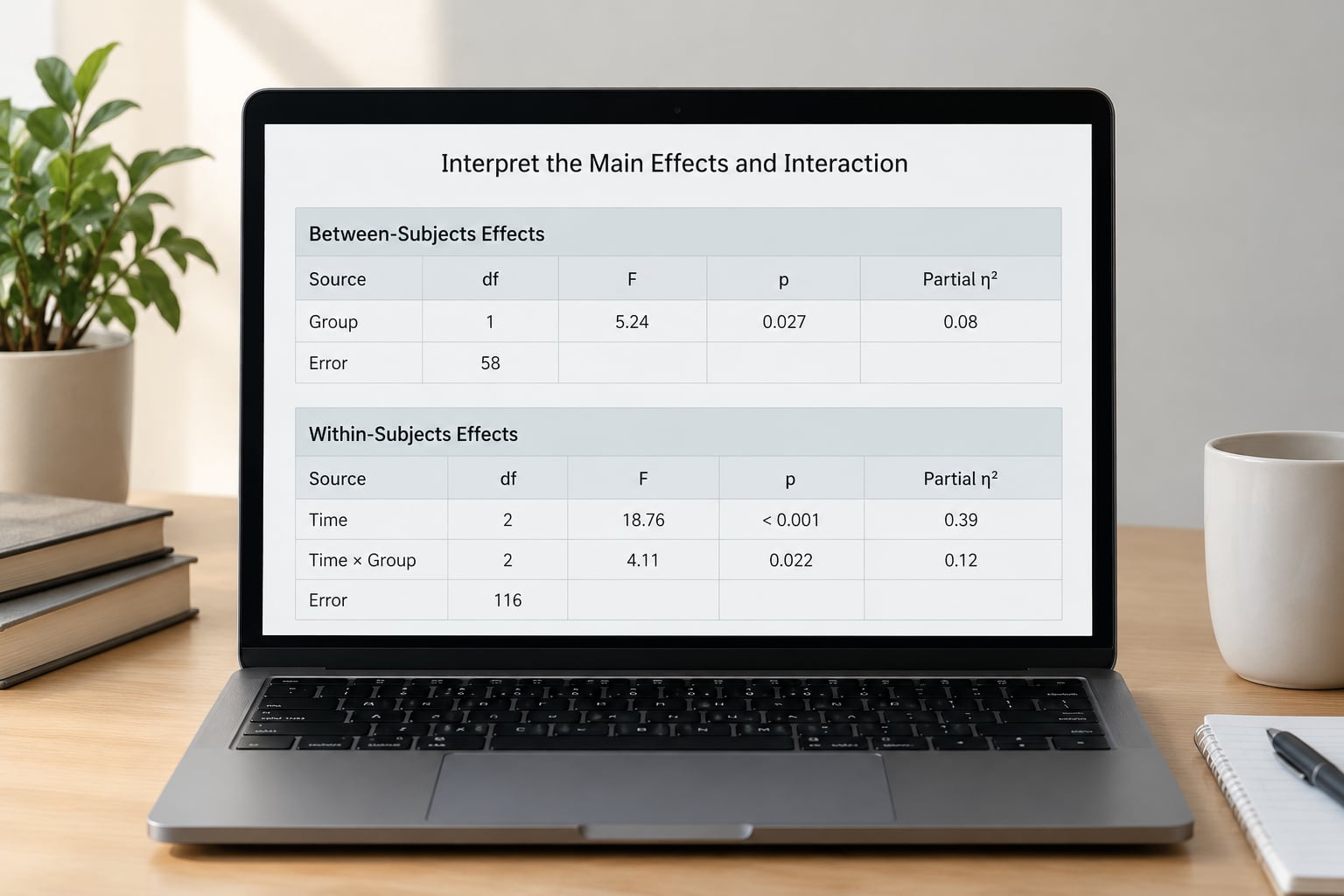
Here is the output from the worked example, with every number derived from the same sums of squares so you can check the arithmetic yourself.

Tests of Within-Subjects Effects

Source	Type III SS	df	MS	F	p	Partial eta squared
time	40.000	2	20.000	22.00	< .001	.500
group * time	24.000	2	12.000	13.20	< .001	.375
Error (time * id within group)	40.000	44	0.909

Mauchly’s test of sphericity for time gave W = 0.782, df = 2, p = .041, so sphericity is violated. Greenhouse-Geisser epsilon was 0.72 and Huynh-Feldt epsilon was 0.79; with epsilon under 0.75 the Greenhouse-Geisser correction is the one to report. Corrected degrees of freedom are 2 x 0.72 = 1.44 for the numerator and 44 x 0.72 = 31.68 for the denominator, giving F(1.44, 31.68) = 22.00 and F(1.44, 31.68) = 13.20.

Tests of Between-Subjects Effects

Source	Type III SS	df	MS	F	p	Partial eta squared
group	30.000	1	30.000	10.00	.005	.313
Error	66.000	22	3.000

Levene’s test was p = .318, so variances are homogeneous. Partial eta squared comes from the SS ratio: 40/(40+40) = .500 for time, 24/(24+40) = .375 for the interaction, and 30/(30+66) = .313 for group.

What those numbers mean

The interaction is significant with a large effect. Scores changed differently across time in the two groups, which is the finding your intervention hypothesis predicted. Partial eta squared of .375 is a large effect by the usual benchmarks.

Read the interaction first, then the main effects. When an interaction is significant, the main effects are averages across levels that the interaction has already shown to be different, so reporting them alone misleads. The main effect of time (F(1.44, 31.68) = 22.00, p < .001) tells you scores rose overall, and the main effect of group (F(1, 22) = 10.00, p = .005) tells you the groups differed overall — but neither tells you how, and the descriptive means show they started nearly level (52.4 against 53.8) and finished far apart (63.7 against 56.9). That is a genuine difference in change, not a pre-existing difference between arms.

Effect size benchmarks used by most textbooks: partial eta squared of .01 is small, .06 is medium and .14 is large.

Unpacking the interaction

A significant interaction is not a result, it is a prompt for simple effects. The estimated marginal means table gives you the numbers to compare, and the profile plot gives you the shape — parallel lines mean no interaction, lines that cross or fan out mean an interaction.

1. Check whether the within effect differs by group: run time within intervention, and time within control, separately. Both effects here would be significant given the size of the divergence.
2. Compare groups at each time point. Pre-test should show no difference; post-test should show one. Adjust for the three comparisons with Bonferroni, giving alpha = .05 / 3 = .0167.
3. Report the simple comparisons with their adjusted p values rather than the raw ones.

If the interaction is not significant, say so plainly and move to the main effects. It does not prove the groups behaved identically; it means the data did not give you enough evidence to claim a difference in change. With a partial eta squared of .02 and p = .31, “there was no evidence of a group by time interaction, F(1.44, 31.68) = 1.09, p = .31, partial eta squared = .02, so main effects are interpreted as the primary results” is a defensible sentence. A non-significant result does not let you skip reporting the interaction at all.

7. Report the Results and Save the Output

Report in this order: assumption checks, then the within-subjects main effect, then the interaction, then the between-subjects main effect, then simple effects if you ran them. APA 7 wants Type III sums of squares when designs are unbalanced.

Copy-paste templates:

A Mauchly's test indicated that the assumption of sphericity was
violated for the within-subjects effect of time, W = 0.78, df = 2,
p = .041, Greenhouse-Geisser's epsilon = .72. Degrees of freedom were
corrected with Greenhouse-Geisser.

A mixed-design ANOVA showed a significant interaction between group
and time, F(1.44, 31.68) = 13.20, p < .001, partial eta squared =
.375. There was also a significant main effect of time,
F(1.44, 31.68) = 22.00, p < .001, partial eta squared = .500, and
a significant main effect of group, F(1, 22) = 10.00, p = .005,
partial eta squared = .313.

One open parenthesis, one closed. Italicise F, p and the statistical symbols, and give the exact p value rather than “p < .05” unless p really is below .001.

Save four things alongside the analysis and label them clearly: the data file used, the syntax file (in SPSS, File > Save As, type .sps), the full unedited output as an .spv file, and your assumption-check notes. If your supervisor asks why you chose Greenhouse-Geisser over Huynh-Feldt, that last item has the answer. Keep the profile plot too — reviewers frequently ask what the interaction looked like, and the plot is the fastest way to show them.

Common Mistakes

1. Treating repeated observations as independent. This is the one that gets work rejected. It inflates the within-subjects error and makes the group difference look stronger than it is. Fix: declare the factor as within-subjects in the Repeated Measures dialog and use Error(id/time) in R.
2. Using the wrong sphericity correction. Reporting uncorrected degrees of freedom after Mauchly’s test came back significant is a straightforward error. Fix: apply Greenhouse-Geisser below epsilon of 0.75, Huynh-Feldt at 0.75 and above, and say which one you used and why.
3. Decoding a between factor as within. If control participants somehow have a “control” value in every time column, they are still one group of people, not three. Fix: classify each factor by asking whether every participant experienced every level before you look at the column names.
4. Reading a non-significant interaction as proof of no interaction. Failure to reach significance is not evidence of equivalence, and reporting it as though the groups are provably alike is a common examiner complaint. Fix: report the F, p and effect size, and say the evidence was insufficient.
5. Reporting p values alone. With roughly 12 participants per cell a small effect can reach significance by luck. Fix: always add partial eta squared, and treat anything under .06 as weak regardless of p.
6. Ignoring the interaction when it is the hypothesis. Running the analysis, finding a significant group main effect and stopping there skips the effect that actually answers the research question. Fix: interpret interaction first.
7. Forgetting listwise deletion. SPSS drops the whole participant when any time point is missing. Fix: check the N in the output against the N you recruited, and report how many cases were excluded.
8. Leaving estimated marginal means unrequested. Without them you cannot compute simple effects without going back and rerunning. Fix: request EMMs in step 7 above, before you click OK.

One more decision worth making deliberately. A mixed ANOVA assumes balanced groups, complete data and one error term for the between factor. If your groups are badly unbalanced, more than about 10% of cases have missing time points, or participants contribute unequal numbers of observations, move to a linear mixed-effects model. It handles all three, uses the same F tests for the fixed effects, and is what experienced reviewers ask for in those situations.

Frequently Asked Questions

Conclusion

Three actions, in order. Classify each factor by asking whether every participant experienced every level, and write the answer down before opening the software. Arrange your data so one row is one participant, with a separate column per within-subjects level. Then check the assumptions — Levene’s test for the between factor, Mauchly’s test for every within effect with three or more levels — and apply Greenhouse-Geisser when Mauchly’s test comes back significant.

After that the analysis itself takes a few minutes, and the reporting template above covers what a supervisor will ask for. This workflow holds for 2026 studies using any current version of SPSS, and the R, Python and Stata code gives you the same model to cross-check against.