
Hierarchical regression lets you enter predictors in blocks, then measure what each new block adds on top of everything already in the model. R square change (ΔR²) is that addition: the new R² minus the old R². If you want to know how to run hierarchical regression and interpret r square change properly, the block F-test (SPSS calls it Sig. F Change) is what tells you whether the increment is real or just noise. Updated for 2026.
Most people get the mechanics right and then misread the output, usually because four different numbers sit in the Model Summary table and only one of them answers “does this block earn its place?”
Table of Contents
- 1What You Need to Run Hierarchical Regression and Interpret R Square Change
- 2Step-by-Step
- 31. Define the Outcome Variable and Predictor Blocks
- 42. Run the Baseline Regression Model
- 53. Add the Next Predictor Block
- 64. Test Whether the New Block Adds Significant Explanatory Power
- 75. How to Calculate and Interpret R Square Change
- 86. Report the Hierarchical Regression in APA Style
- 9Common Mistakes
- 10Frequently Asked Questions
- 11How many predictor blocks should a hierarchical regression have?
- 12Can I use hierarchical regression with categorical or interaction predictors?
- 13What does it mean if R square change is small but statistically significant?
- 14Should I enter all predictors in one block if I only need the final R squared?
- 15Can I run hierarchical regression in R or Stata instead of SPSS?
- 16What sample size is required for hierarchical regression?
- 17Conclusion
What You Need to Run Hierarchical Regression and Interpret R Square Change
You need four things lined up before you open the software, and the first two do more work than the software does.
- An outcome variable that is continuous, or a reasonable numeric stand-in for a construct. If you are scoring a survey, decide whether to use the scale total or the mean before you model anything, not after.
- Predictor blocks with a defensible order. Block 1 usually holds the variables you need as controls or nuisance factors. Later blocks hold the theoretical variables you actually care about.
- A dataset with missing values already dealt with. Every case in the analysis must have complete data on every variable in every block, or SPSS drops it silently and your sample shifts between blocks.
- A sample that can carry the model. The old rule of thumb is 15 to 20 complete cases per predictor. With three blocks and eight predictors, that is a sample in the 120 to 160 range before you even think about interaction terms.
Block order is the part people rush, and it is the part that decides what your results mean. There are three conventions worth knowing, and they get cited constantly in methods sections.
- Time precedence. Enter first the variables that causally precede the others. Sleep before stress before burnout, for instance.
- Manipulability. Enter the predictor you could realistically intervene on before the ones you cannot.
- Perceived importance. When the first two do not apply, enter what your field treats as the most important predictor first.
Different software does block entry differently, so it helps to know the equivalent commands before you switch tools.
| Software | How blocks are specified | Where the block test comes from |
|---|---|---|
| SPSS | Analyze > Regression > Linear, with a built-in Block 0 / Next structure | Sig. F Change and F Change in the Model Summary table |
| R | Fit one lm() per nested model, then compare with anova() | The anova() comparison row for the added terms |
| Python (statsmodels) | Fit one OLS per nested model, compare with anova_lm(..., typ=1) | The Pr(>F) value on the comparison row |
| Stata | Run each regress in turn, or use the nestreg prefix for a formatted table | Model F and the nested model comparison; pcorr if you need a semi-partial |
In R the whole sequence is three lines, which is genuinely quicker than clicking through SPSS dialogs once you have done it twice.
m1 <- lm(score ~ attendance + gpa, data = d)
m2 <- lm(score ~ attendance + gpa + hours, data = d)
anova(m1, m2)
The Python equivalent uses sequential sums of squares, which is what SPSS’s block test is doing under the hood.
import statsmodels.formula.api as smf
import statsmodels.api as sm

m1 = smf.ols("score ~ attendance + gpa", data=d).fit()
m2 = smf.ols("score ~ attendance + gpa + hours", data=d).fit()
print(sm.stats.anova_lm(m1, m2, typ=1))
Step-by-Step
1. Define the Outcome Variable and Predictor Blocks
Write the block order on paper before you touch the software, and write down the reason for each block. Reviewers ask for that justification, and it protects you from the most damaging critique in this whole area: blocks chosen after seeing the data.
Three kinds of variables tend to appear. Controls are nuisance variables such as age, gender, or site. Contextual variables describe the situation the outcome occurred in. Substantive variables are the theoretical stars, usually entered last so their unique contribution is visible.
Check your effective sample size before modelling. Look at the missing-values table, decide your listwise deletion rule, and confirm the remaining N is still at least 15 to 20 per predictor. Also inspect the distributions of your continuous predictors now, because a skewed scale entered later will make the regression assumptions painful to untangle.
2. Run the Baseline Regression Model
In SPSS, the path is Analyze > Regression > Linear. Put your outcome in the Dependent box. The first set of predictors goes in Block 0, which SPSS treats as the baseline model.
Open the Statistics button and tick Estimates, Model fit, Descriptives, Casewise diagnostics, Collinearity diagnostics, Residual plots, and the Normal probability plot of standardised residual. R square change is not optional in SPSS; it is always reported.
When you click OK, read four rows from the Model Summary table for Block 1: R, R Square, Adjusted R Square, and Std. Error of the Estimate. Then open the Coefficients table and note the unstandardised B, standardised beta, t, and Sig. columns for each predictor.
Stop and fix things before adding anything if the diagnostics look wrong. Collinearity diagnostics matter most here: tolerance below .10 or a variance inflation factor above 10 is a red flag, and a condition index above 30 means serious multicollinearity. Correlations between two predictors above .80 also deserve a second look. Fixing this later is far harder than fixing it in Block 1.
3. Add the Next Predictor Block
Click Next in the dialog. SPSS opens Block 1 and gives it a name, which you should change from “Block 1” to something descriptive like “Controls” or “Study behaviour”. Type your new predictors into the second box and click Next again for each further block.
Nothing about this step is automated. SPSS is not choosing variables by their contribution to the model; it enters them in the order you specified. That is the whole difference between hierarchical regression and stepwise regression, where the software adds and removes terms based on the data alone. Stepwise answers “what predicts best in this sample.” Hierarchical answers “does this block add anything once I already account for that?”
4. Test Whether the New Block Adds Significant Explanatory Power
Three tables matter here, and they answer different questions.
The Model Summary table tells you the size of the fit and the size of the increment. The ANOVA table gives the overall F for the whole model plus the F Change row for each block. The Coefficients table gives you the individual predictors.
The row to read is F Change, with its Sig. F Change value. If Sig. F Change is below .05, the new block explains a meaningful share of variance that the previous blocks did not, and you can say the block adds significant unique variance. If it is above .05, the block did not improve the model.
A common misreading is treating a nonsignificant F Change as proof that nothing in the block relates to the outcome. It is not. It means the block’s variables, taken together, did not add explanatory power above what came before. Individual predictors in that block can still be significant, and often are, because a block F test is a joint test of several coefficients.
5. How to Calculate and Interpret R Square Change
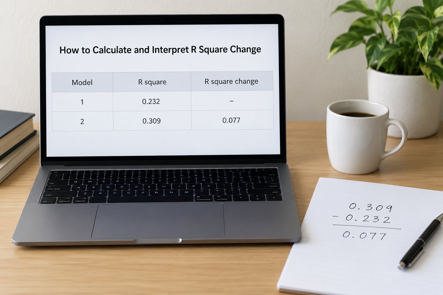
The calculation itself is subtraction. Take the R² of the full model and subtract the R² of the model that stopped one block earlier.
Here is a complete worked example, using 150 students with a final exam score as the outcome. Block 1 is attendance rate and prior GPA. Block 2 adds weekly study hours outside class. Block 3 adds a self-efficacy by study hours interaction.
| Model | R | R Square | Adjusted R Square | Std. Error | Change in R Square | Change in Adjusted R Square | F Change | Sig. F Change |
|---|---|---|---|---|---|---|---|---|
| 1 Controls | .482 | .232 | .222 | 8.82 | 22.20 | .000 | ||
| 2 + Study hours | .556 | .309 | .295 | 8.40 | .077 | .073 | 16.36 | .001 |
| 3 + Interaction | .604 | .365 | .347 | 8.08 | .056 | .052 | 12.88 | .001 |
Block 2’s change in R square is .309 minus .232, which is .077. Read that as seven point seven percentage points of variance in exam score that study hours explain, and attendance plus prior GPA do not. The full model explains 30.9 percent of the variance, up from 23.2 percent.
Sig. F Change of .001 tells you that increment is unlikely to have appeared by chance, with F(1, 147) = 16.36. Block 3 adds a further 5.6 points and is also significant, F(1, 146) = 12.88, p = .001.
Four numbers appear in that table, and mixing them up is the single most common error in this analysis. Here is how to tell them apart.
| Number | What it measures | How to use it |
|---|---|---|
| R² | Total variance the current model explains | Descriptive. Report it for the final model. |
| Adjusted R² | R² penalised for the number of predictors | The fairer fit comparison across models with different predictor counts. |
| ΔR² | Extra variance the new block explains | The size of the block’s unique contribution. |
| ΔAdjusted R² | The same increment, after the penalty | Can be negative. If it is, the block cost you more than it gave. |
Adjusted R² is computed as 1 minus (1 minus R²) multiplied by (n minus 1) and divided by (n minus p minus 1), where n is your sample size and p the number of predictors. It always sits below R² once you have more than one predictor, and the gap widens as predictors pile up.
When adjusted R² drops across blocks, that is not a crisis. It means the new variables explained less variance than the statistical penalty charged for adding them. Test the block on Sig. F Change rather than on adjusted R², and report both honestly.
Is .077 a big change? There is no universal threshold, and any article claiming one is overselling. Context decides. An additional 7.7 percent is substantial for a second block in education or organisational research and unremarkable in machine learning. Compare it against what you expected to gain and against the zero-order correlation between the new block and the outcome.
That zero-order comparison is a useful ceiling. Study hours correlate with exam score at roughly r = .34, and squaring gives r² = .116, so study hours could never explain more than 11.6 percent of the outcome on their own. Realising .077 of that .116 means most of the available signal survived the controls. The formal upper bound is the squared semi-partial correlation, which you can get in Stata with pcorr. When the semi-partial comes out near zero while the zero-order correlation is respectable, you are looking at suppression, and no amount of reordering will fix it.
6. Report the Hierarchical Regression in APA Style
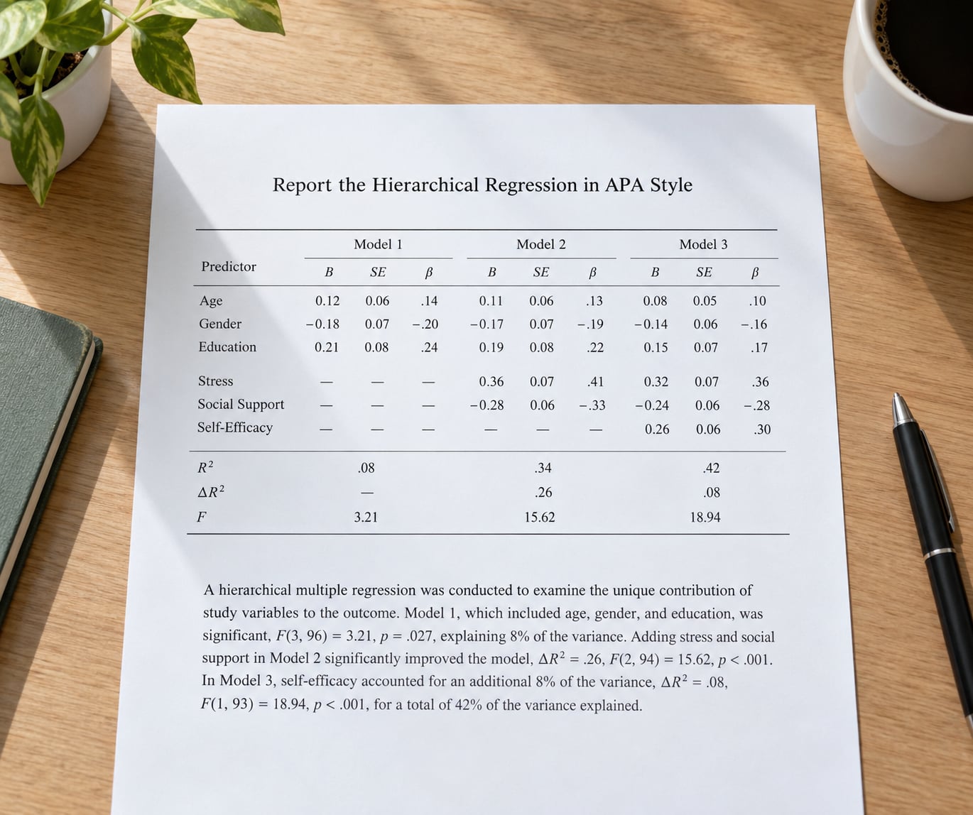
APA style reports the models as columns, not as separate tables. Each column is one model in the sequence, which is exactly what your Model Summary table already contains.
| Predictor | M1 | M2 | M3 |
|---|---|---|---|
| Attendance rate | .34*** | .29*** | .21*** |
| Prior GPA | .27*** | .23*** | .19** |
| Study hours | .26*** | .18** | |
| Self-efficacy x hours | .18*** | ||
| R² | .23 | .31 | .37 |
| Adjusted R² | .22 | .30 | .35 |
| ΔR² | .08 | .06 | |
| F change | 22.20*** | 16.36*** | 12.88*** |
Then write the paragraph in full sentences, which is where most marks are lost.
A hierarchical regression was conducted in which attendance rate and prior GPA were entered in Block 1, followed by weekly study hours in Block 2 and the self-efficacy by study hours interaction in Block 3. Attendance rate and prior GPA explained 23.2 percent of the variance in final exam score, F(2, 147) = 22.20, p < .001. Adding study hours significantly improved the model, ΔR² = .077, F(1, 147) = 16.36, p = .001, and the full model accounted for 30.9 percent of the variance. The interaction term added a further 5.6 percent, ΔR² = .056, F(1, 146) = 12.88, p = .001, taking the model to 36.5 percent.
Three habits keep this clean. Round R², ΔR², and betas to two decimals, and never round a p value below .001. Use the word “predicted” rather than “caused” unless the design genuinely supports a causal claim. And if Sig. F Change is nonsignificant, say the block did not improve the model rather than reaching for a softer phrase that implies it nearly did.
One diagnostic worth reading while you write the table is coefficient shrinkage. Attendance drops from a beta of .34 in Block 1 to .29 in Block 2 and .21 in Block 3. Large shrinkage means your blocks share variance with each other, which is exactly what controls are supposed to do, but severe shrinkage alongside a small ΔR² is a hint that your controls may be absorbing the very effect you are trying to measure.
Common Mistakes
Changing the model to chase a bigger R². Moving a predictor from one block to another until the increment looks good invalidates the whole design. Fix the order from theory, then leave it alone.
Reading ΔR² as the final R². In the example above, .077 is the increment, not the model’s explanatory power. The model explains .309. Confusing the two is the most common reporting error in published papers.
Treating a causal claim as proven. Block entry controls for variance statistically. It does not neutralise unmeasured confounders, and it never converts observational data into an experiment.
Entering blocks after seeing the outcome. Once you know which variables produced the result, the ordering is no longer independent. Either justify the order from theory or, if no theory exists, run every plausible sequence and report the range of results instead of one number.
Calling a nonsignificant block proof of no relationship. Sig. F Change above .05 says the joint contribution was not detectable in this sample. With a small sample, that is a power problem, not a finding.
Skipping multicollinearity and interaction checks. Product terms inflate collinearity badly, so mean-centre your variables before you build the interaction term. That keeps the intercept interpretable and the main effects meaningful, which is the resolution most researchers land on after debating whether to centre or standardise.
Frequently Asked Questions
How many predictor blocks should a hierarchical regression have?
Two or three is the usual range, and that is usually enough. Each block needs a clear theoretical job: controls first, then the variables you most want to test, then any interaction or moderation term. More blocks add reporting complexity without adding clarity, and splitting a block into small pieces makes the incremental F tests underpowered. If you find yourself with six blocks, ask whether some of those variables belong together.
Can I use hierarchical regression with categorical or interaction predictors?
Yes, both work, with one preparation step for interactions. Categorical variables with more than two levels need dummy coding, and the usual convention is to drop one category as the reference group. For interaction terms, mean-centre all the variables involved before creating the product term. Centring leaves the interaction effect itself unchanged but makes the intercept and main effects interpretable, which saves a lot of confusion later.
What does it mean if R square change is small but statistically significant?
It means the block adds a small but detectable amount of unique variance. With a large enough sample, even a small increment can clear the significance threshold, so a small ΔR² with p below .05 is not a contradiction. What you write depends on your field: state that the block added significant unique variance, give the exact ΔR² and F value, and avoid describing the effect as large. Sample size and effect size are answering different questions here.
Should I enter all predictors in one block if I only need the final R squared?
Technically you can, and the final R² will be the same either way. You lose the ability to say how much any group of variables contributed, and you gain nothing in terms of accuracy. The reason to keep blocks separate is interpretive: without them you cannot answer whether your theoretical variable matters beyond the controls, which is usually the actual question behind the analysis.
Can I run hierarchical regression in R or Stata instead of SPSS?
Yes. In R, fit one lm() model per nested formula and compare them with anova(), which returns the F test for the added terms. In Stata, run each regress in sequence, or use nestreg for a formatted nested table, with pcorr when you need the significance of a specific coefficient. Both give you the block test SPSS reports as Sig. F Change.
What sample size is required for hierarchical regression?
The working rule is 15 to 20 complete cases per predictor in the final model, including any dummy variables and interaction terms. If you are testing whether a block adds a small increment, that rule is not generous enough, because incremental tests carry less power than the overall model test. Power analyses based on the specific effect you hope to detect are worth the effort, and they usually call for a larger sample than people expect.
Conclusion
Start by writing down your outcome and your theoretically ordered blocks, then run the baseline model and check its diagnostics before adding anything. Once the blocks are in, read Sig. F Change for the verdict, ΔR² for the size of the contribution, and adjusted R² for the honest fit comparison. Report all three and describe what the block adds above the controls, never what it caused.