How to Run a Two Way ANOVA in SPSS With Interaction (October 2026)

To run a two way anova in SPSS with interaction, open Analyze > General Linear Model > Univariate, drop your continuous outcome into the Dependent List, move both categorical factors into the Fixed Factor(s) box, and keep Model set to Full Factorial so the interaction term is estimated. From there you read one table — Tests of Between-Subjects Effects — and start with the interaction row, not the main effects.

The interaction is the part people skip, and it is the part that decides how you are allowed to write up the rest. If it is significant, the average effect of each factor on its own is misleading, and reporting those two main effects anyway is the single most common statistical error supervisors send back.

This walkthrough uses IBM SPSS Statistics on Windows and macOS. The dialog is identical across recent versions, and older releases put the same procedure under Analyze > Compare Models > Two-Way ANOVA. Give yourself about twenty minutes for a first run, most of which is checking your data rather than clicking.

Table of Contents

1. 1What You Need: Three Variables and Data in Every Cell
2. 2Step-by-Step: How to Run a Two Way ANOVA in SPSS With Interaction
3. 3Check and Prepare Your Data
4. 4Open the Two-Way ANOVA Dialog
5. 5Assign the Dependent Variable and Factors
6. 6Select Model, Main Effects, and Interaction
7. 7Run the Analysis and Check the Output
8. 8The UNIANOVA Syntax Behind Those Clicks
9. 9Interpret the Main Effects and Interaction
10. 10Report the Results in APA Style
11. 11Common Mistakes
12. 12Tips for Reliable Results
13. 13Frequently Asked Questions
14. 14Do I include the interaction in a two-way ANOVA in SPSS?
15. 15What does a significant interaction mean in a two-way ANOVA?
16. 16Should I use balanced or unbalanced samples for two-way ANOVA?
17. 17What should I do if Levene’s test is significant in SPSS?
18. 18Which post-hoc tests can I use after a two-way ANOVA?
19. 19How do I report a two-way ANOVA interaction in APA style?
20. 20Conclusion: Check Your Factors, Run Full Factorial, Read the Interaction First

What You Need: Three Variables and Data in Every Cell

You need two categorical independent variables, one continuous dependent variable, and a dataset where each participant supplies one value for the outcome.

Both factors must be nominal or ordinal with real categories. A factor is a variable whose values name groups — treatment type, site, gender, difficulty level — not something measured on a continuous scale. Age in years is not a factor; age band such as 18-29, 30-44 and 45+ is.

The dependent variable goes on the scale measurement level: test score, reaction time, weight, symptom count treated as continuous.

You also need data in every cell of the design. A 2×3 design has six cells, and the interaction is only estimable when each of them holds scores from several participants. A cell with a single case cannot contribute an estimate, and SPSS will either warn you or quietly produce an error term you should not trust.

Decide whether your design is between subjects. If every participant appears in exactly one combination of the two factors, it is a between-subjects design and the Univariate procedure is correct. If the same participants supply scores under every level of one factor, that factor is a within-subjects factor and you need Analyze > General Linear Model > Repeated Measures instead, where the interaction gets its own within-subjects effects table.

Finally, decide whether your cells are balanced. Balanced means the same number of participants in each cell. SPSS handles unbalanced designs, but it will use Type III sums of squares rather than Type I, and you should report that choice rather than leaving it unsaid.

Step-by-Step: How to Run a Two Way ANOVA in SPSS With Interaction

Check and Prepare Your Data

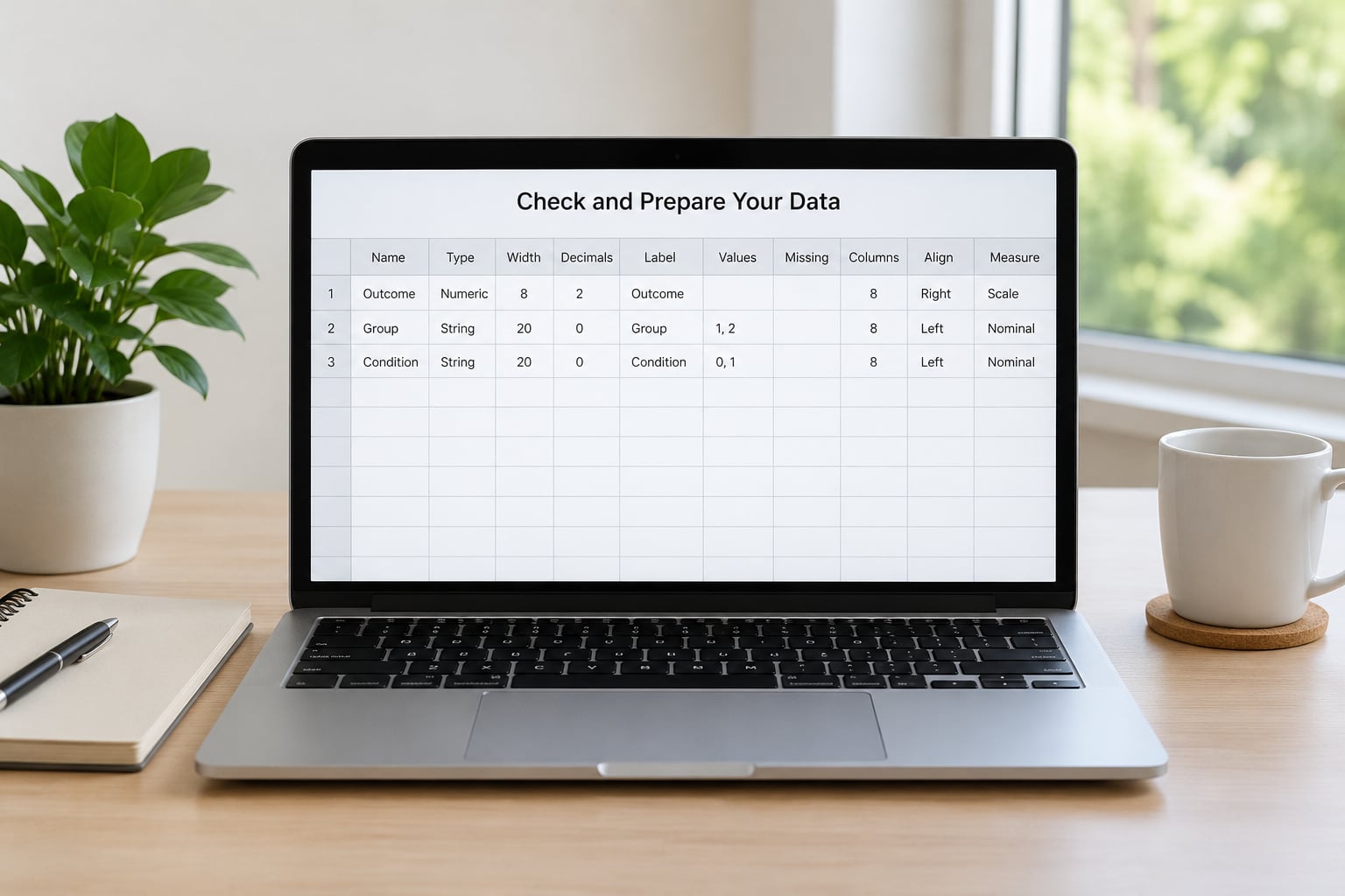
Open Data > Sort Cases and order rows by one factor, then the other, so the design is easy to eyeball.

Switch to the Variable View tab and check three things on each column. The Measure cell must read Nominal or Ordinal for both factors and Scale for the dependent variable. Values must be coded consistently, with no factor mixing numbers 1, 2, 3 with words like yes and no.

Add value labels through the Labels column so the output shows readable group names rather than bare codes. This matters more than it sounds, because the interaction row in the output is labelled with whatever codes your factors carry.

Look for missing data. Data > Select Cases > If condition is not complete will drop rows with gaps from the analysis. Choose that deliberately and note the count in your write-up, because silent listwise deletion changes your cell sizes.

Count the cells before you analyse anything. Run Data > Compare Files > Crosstabs, put each factor in Rows and Columns, click Statistics and tick Chi-square, then look at the Count cells in each quadrant. That table tells you whether the design is balanced and how many cases you actually have per cell.

Open the Two-Way ANOVA Dialog

Go to Analyze > General Linear Model > Univariate. That is the full path in current versions of IBM SPSS Statistics.

In SPSS releases before about version 20 the procedure lives at Analyze > Compare Models > Two-Way ANOVA. The two dialogs look different but produce the same model and the same Tests of Between-Subjects Effects table, so a screenshot from an older tutorial will not mislead you about the statistics.

If you want a one-paragraph summary to get you moving: open Univariate, place the continuous outcome in the Dependent List, place both categorical factors in Fixed Factor(s), confirm Model is Full Factorial, request descriptives and effect sizes under Options, then click OK.

Assign the Dependent Variable and Factors

Click your outcome variable once, then click the arrow next to Dependent List to move it in.

Select the first factor, holding Ctrl for the second, and move both into Fixed Factor(s). Fixed Factor(s) is the correct box for group variables you manipulated or want to compare. Dependent Variable would treat your groups as the outcome.

The order you add them does not change the test. SPSS names the first factor you place factor1 and the second factor2, and everything downstream — the interaction row label, the profile plot axes — follows that order. Swapping them flips which variable sits on the horizontal axis of the profile plot and nothing else.

Check the little assigned variable box above the list. It should show one variable ending in an asterisk next to each other, for example diet * exercise. That asterisk is the interaction term, and if it is missing, your model does not contain it.

Select Model, Main Effects, and Interaction

Click Model… and confirm the selected radio button is Full Factorial. This is the setting most people get wrong.

Full Factorial estimates the two main effects and the interaction together. Main effects only runs two separate one-way models, and the output will contain no interaction row at all — no error message, just a missing line in the table. Main effects only is the right choice in exactly one situation: when you have already decided, before seeing the data, that the interaction is not of interest.

In the Model dialog you can also build custom models by clicking the Paste button. Typing A B A*B reproduces the full factorial model by hand, which is a useful check that you know what the software is fitting.

Before you run anything, click Paste… at the bottom of the main dialog. SPSS writes your whole analysis into a syntax window, and the design line at the end tells you the truth: /DESIGN = diet exercise diet*exercise. If the interaction is not on that line, the analysis will not test it.

Run the Analysis and Check the Output

Before clicking OK, set the four sub-dialogs so the output answers your questions the first time.

In Options, tick Descriptives, Effect size estimates, Homogeneity tests and Intercept. That single step produces the descriptive statistics table, the partial eta squared column, and Levene’s test without a second run.

In Plots, move the factor you want on the horizontal axis to Horizontal axis, the other to Separate lines, and add the interaction by putting both factor names in the box below, again separated by an asterisk. This produces the profile plot.

In Post Hoc, select the factor whose levels you intend to compare pairwise and apply Tukey. Only do this for a main effect that turns out to be interpretable. Applying post hoc tests to a factor whose interaction is significant tells you nothing useful and invites criticism.

In EM Means, tick Display Mean for both factors and both together. Estimated marginal means are the averages SPSS computes after fitting the model, and they are what you graph and report for simple effects.

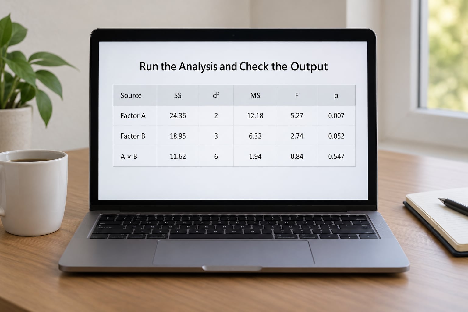
Click OK and look for the Tests of Between-Subjects Effects table. It should list a Corrected Model row, an Intercept row, one row per main effect, one row for the interaction, and an Error row.

Check three other tables while you are in there. Levene’s Test of Equality of Variances tells you whether homogeneity held. Descriptive Statistics gives you the raw cell means, which you can compare against the estimated marginal means. The profile plot shows whether the lines are parallel or crossing.

The UNIANOVA Syntax Behind Those Clicks

Every box you just filled maps to a line of syntax. Pasting it gives you a reproducible command file, which matters if your supervisor asks how the analysis was run rather than wanting a screenshot of it.

UNIANOVA outcome BY diet exercise
  /METHOD = SSTYPE(3)
  /INTERCEPT = INTERCEPT
  /PLOT = PROFILE(factor1*factor2)
  /EMMEANS = TABLES(diet*exercise)
  /POSTHOC = diet(experiment) TUKEY
  /PRINT = DESCRIPTIVE ETASQ HOMOGENEITY
  /DESIGN = diet exercise diet*exercise.

Read the /DESIGN line as the sentence the whole analysis rests on: both main effects plus their product term. If the interaction is not there, it is not being tested. SSTYPE(3) is the Type III sums of squares SPSS uses by default, and you should name it in your write-up when your cells are unbalanced.

When the interaction is significant, add a COMPARE line to /EMMEANS and end it with the adjustment you want. This is the part no page-one tutorial spells out, and it is the line that gives you within-cell comparisons:

UNIANOVA outcome BY diet exercise
  /METHOD = SSTYPE(3)
  /INTERCEPT = INTERCEPT
  /PLOT = PROFILE(factor1*factor2)
  /EMMEANS = TABLES(diet*exercise)
    COMPARE(diet) ADJ(BONFERRONI)
    COMPARE(exercise) ADJ(BONFERRONI)
  /PRINT = DESCRIPTIVE ETASQ HOMOGENEITY
  /DESIGN = diet exercise diet*exercise.

Bonferroni is strict, which is the point. Each level of the blocking factor gets its own set of comparisons, so without an adjustment the Type I error rate climbs quickly across cells. If your design is mixed or within subjects, the same logic applies but the command changes to GLM REPEATED, and the interaction is estimated through /DESIGN with the within-subjects factor syntax instead.

Interpret the Main Effects and Interaction

Read the interaction row first. Everything after it depends on what that row says.

Each row gives you an F statistic, degrees of freedom, a Sig. (p) value, and a partial eta squared. p below .05 means reject the null for that effect. Partial eta squared describes size on a 0 to 1 scale; .01 is a small effect, .06 a medium one, .14 a large one.

A significant interaction means the effect of factor A is not the same at every level of factor B. The words students need are simple: the difference between the groups on A changes depending on which group they are in.

Look at the profile plot to make the same point visually. Parallel lines mean no interaction — the gap between groups is the same at both levels of the other factor. Non-parallel lines mean the size of the gap changes with the level. Crossing lines, where the ordering of groups reverses, are the clearest case: the effect even changes sign.

If the interaction is significant, do not report the two main effects as standalone findings. They are averages across conditions that mask the real pattern, and many journals and supervisors treat that as a reporting error rather than a stylistic one. Report the interaction, then run simple effects — comparing factor A separately within each level of factor B.

Simple effects are straightforward once you see what they are. The Compare main effects box inside the EM Means dialog only produces comparisons for the main effects, not inside the interaction cells, which surprises nearly everyone. To get the comparisons you want, use Paste, then edit the syntax so the /EMMEANS line compares the factor against itself within each level of the other, and add a Bonferroni adjustment to hold down Type I error. Alternatively, run separate analyses per level of the blocking factor and let SPSS generate the pairwise tables for you.

If the interaction is not significant, the picture simplifies. The main effects are now interpretable on their own, and for any significant main effect you can move to the Post Hoc table to see which specific pairs of levels differ.

Report the Results in APA Style

Lead with the interaction, then the main effects, then the descriptive statistics.

A significant interaction reads like this: “A two-way ANOVA showed a significant interaction between [factor A] and [factor B], F(df1, df2) = X.XX, p = .XXX, partial eta squared = .XXX. Simple effects analysis showed that the effect of [factor A] was significant at [level 1 of B] … and not significant at [level 2 of B] …”

A non-significant interaction reads like this: “There was no significant interaction between [factor A] and [factor B], F(df1, df2) = X.XX, p = .XXX, partial eta squared = .XXX.” Then report whichever main effects were significant, each with its own F, df, p and partial eta squared.

Keep exact p values to three decimals and omit the leading zero for p and partial eta squared, following APA 7. Report the number of participants and the number of predictors next to each F, for example F(1, 44) for a 2×2 between-subjects design. Check your target journal’s requirements, since some still want exact values rather than p thresholds.

Common Mistakes

No interaction row in the output. The model was set to Main effects only, or the interaction never reached the Fixed Factor(s) box. Reopen Model and choose Full Factorial, then confirm the pasted syntax lists both factors and the interaction.

SPSS refuses to run, or warns about cells. A factor was left on the Scale measurement level, so SPSS is treating it as continuous. Set both factors to Nominal in Variable View.

Main effects reported alongside a significant interaction. The output was read top to bottom instead of interaction first. Drop the standalone main effects and report simple effects instead.

Levene’s test significant, results ignored. The homogeneity row was never requested in Options. Report the violation openly, and consider a Welch-type approach or bootstrapping, or reformulate the outcome as one that meets the assumption.

Only p values in the write-up. Effect size estimates were never requested. Tick Effect size estimates in Options and report partial eta squared alongside every F.

Cells look unbalanced in the output. Different numbers of participants per cell, or listwise deletion changed them silently. Count the cells with a crosstab before you run, and report Type III sums of squares when the design is unbalanced.

Tips for Reliable Results

Interactions need more participants than main effects do, because the test compares a pattern across cells rather than a single average. If you have fewer than roughly 20 cases per cell, expect the interaction to be underpowered even when a real effect exists, and say so rather than reporting a non-significant result as evidence of nothing.

Check normality per cell, not overall. Explore > Graphs > Histogram with the factor placed in the Panel variable gives you one panel per cell, and the Q-Q plot shows departures from the diagonal clearly enough for a working judgement.

Check for outliers before you run the analysis. Explore > Analyze > Boxplots, or compute a z-score and look for anything beyond about 3. An extreme case in one cell can manufacture an interaction that is really one data point.

Save the syntax every time. After Paste, save the file in your project folder. Supervisors increasingly ask for the command file rather than the output, and a menu-only analysis cannot be reproduced by anyone else.

Use Align on the Plots dialog if your groups are tiny, and never reach for post hoc tests just because the table offers them.

Frequently Asked Questions

Conclusion: Check Your Factors, Run Full Factorial, Read the Interaction First

Start by opening Variable View and confirming both independent variables are measured as Nominal and the dependent variable as Scale. Then run Analyze > General Linear Model > Univariate with Model set to Full Factorial, and read the interaction row in Tests of Between-Subjects Effects before you write a word about either main effect.

That single habit — interaction first, then branching to simple effects or to main effects and post hoc tests — is what separates a defensible results section from one a reviewer queries.

Keep the pasted syntax file next to your output, and revisit the whole procedure when you start a fresh analysis for 2026 coursework or a thesis.