How to Run MANOVA in SPSS and Interpret Output (2026)

If you want to know how to run MANOVA in SPSS and interpret output, the whole procedure lives under Analyze > General Linear Model > Multivariate. You drop two or more continuous dependent variables into one box, put your categorical groups into Fixed Factors, and SPSS returns a single omnibus test of whether the set of outcomes differs across groups. The rest of this guide walks through that click path, then shows you how to read each output table and what to write in your paper.

Two things trip people up before they even start. First, there is no menu item called MANOVA anywhere in SPSS, so searching for it wastes ten minutes. Second, SPSS calls your independent variables “Fixed Factors,” not “Independent Variables,” so students drag the wrong variable into the wrong box and get an error or a meaningless result.

This guide covers the between-groups (independent samples) version of the procedure, which is what most assignments need. Repeated measures MANOVA uses the same dialog with a different setup, and I’ll touch on that near the end. Menu names can shift slightly between older releases, so if your interface looks different, look for the General Linear Model menu and the Multivariate item inside it.

Table of Contents

1. 1What You Need
2. 2Step-by-Step: How to Run MANOVA in SPSS and Read the Output
3. 3How to Run MANOVA in SPSS: Select the Variables
4. 4Check Box M and Other Assumption Tests
5. 5Interpret the Multivariate Tests
6. 6Follow a Significant Multivariate Effect
7. 7Report and Visualize the Results
8. 8Common Mistakes
9. 9Frequently Asked Questions
10. 10Which MANOVA test statistic should I use in SPSS?
11. 11What assumptions should I check before interpreting MANOVA output?
12. 12Why is a univariate ANOVA significant when MANOVA is not?
13. 13What post-hoc test should I use after a significant MANOVA?
14. 14When should I use MANOVA instead of one-way ANOVA?
15. 15Conclusion

What You Need

You need IBM SPSS Statistics (version 29 for Windows or macOS is the current release, and older versions work almost identically) and a dataset in which the variable roles are already sorted out. MANOVA is a General Linear Model procedure, so it expects continuous outcome variables and categorical grouping variables. The two cannot be mixed up.

• Two or more continuous dependent variables. Numeric scores such as reaction time, exam marks, a Likert composite, systolic blood pressure, or monthly spend. SPSS needs more than one, otherwise it is just an ANOVA.
• At least one categorical independent variable with two or more levels. Group, condition, treatment, gender, year cohort, or an experimental arm. These go into Fixed Factors.
• A design where groups are independent of each other. Every participant sits in exactly one group. If the same people are measured repeatedly, that is a different procedure.
• Enough cases per group. The common rule of thumb is that each group should contain more cases than the number of dependent variables. With four dependent variables, aim for at least five cases per group, and considerably more in practice.
• Measured covariates, if you plan to control for them. Age, years of experience, baseline score. Anything numeric that is not an outcome goes into the Covariates box rather than Fixed Factors.

One design note worth knowing before you click anything. MANOVA is not “a two-way ANOVA.” It is the multivariate sibling of the General Linear Model, so it handles one factor, two factors, and three factors with the same dialog. What changes is how many factors you put in the Fixed Factors box and which model terms SPSS builds in the Model dialog. A two-way MANOVA simply means two factors in that box.

Step-by-Step: How to Run MANOVA in SPSS and Read the Output

How to Run MANOVA in SPSS: Select the Variables

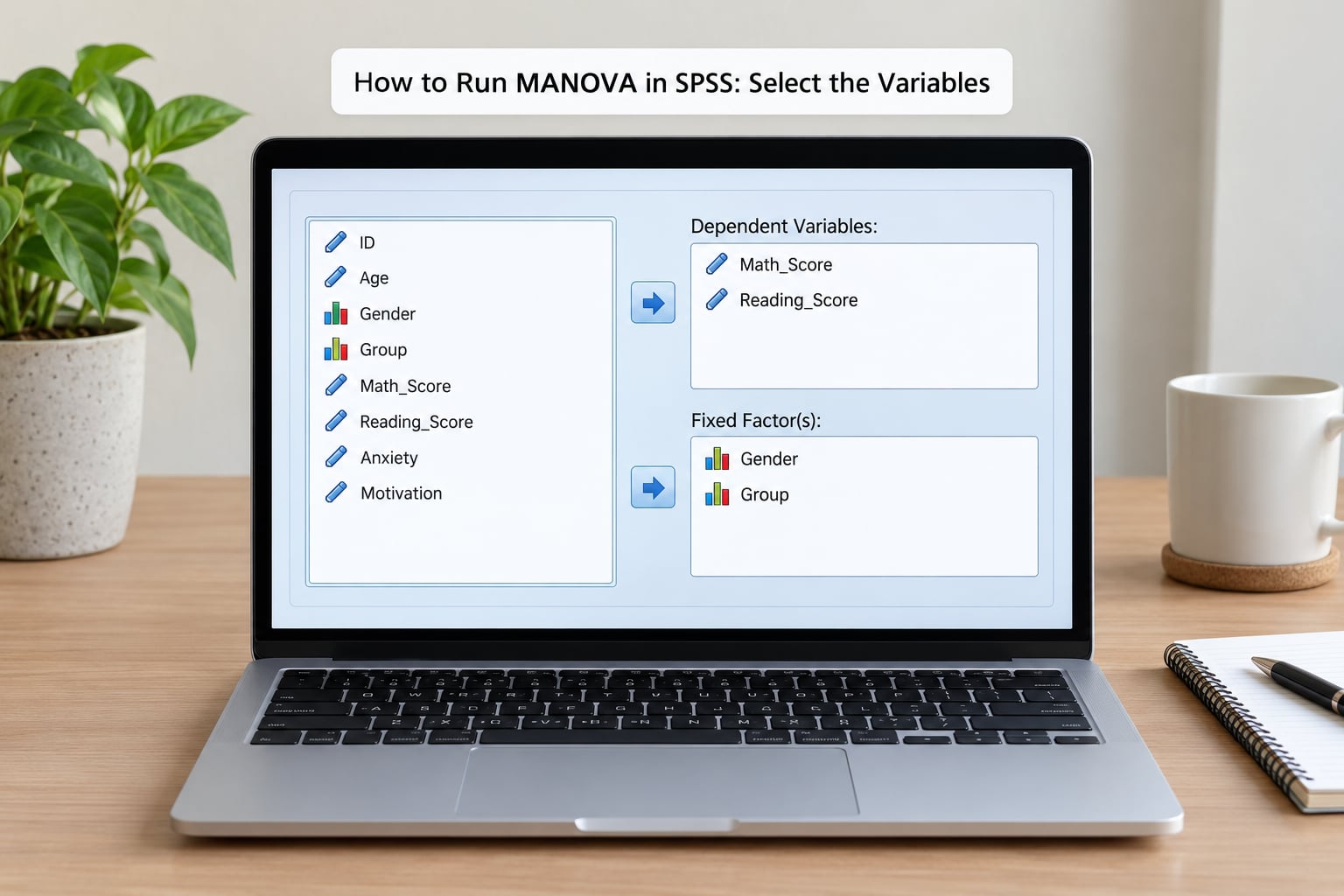
The menu path is Analyze > General Linear Model > Multivariate, and the Multivariate dialog opens with four boxes on the left: Dependent Variables, Fixed Factors, Covariates, and an empty Model box on the right.

1. Check your variables first. Run Analyze > Descriptive Statistics > Frequencies on each dependent variable, or at minimum look at the missing values in the Variable View. Missing cases are handled case-by-case, so a few blanks quietly shrink your N in ways you will want to explain later.
2. Move your outcomes into Dependent Variables. Select them all, then click the arrow into the top box. SPSS accepts multiple variables here, which is exactly what separates MANOVA from univariate ANOVA. If you put only one variable there, you are running an ANOVA and no amount of significance will change that.
3. Move your grouping variable into Fixed Factors. This is the step beginners miss. The label says Fixed Factors, not Independent Variables. The variable must be categorical, so check Data View and confirm the Measure column reads “Nominal.” A numeric group code stored as Scale will not go here.
4. Add covariates if you need them. Numeric variables you want to control for go into Covariates. Keep it simple: more than one or two covariates on a small sample will give you unstable results and meaningless estimated marginal means.
5. Click Model to confirm the terms. By default SPSS builds an intercept plus the main effect of each factor. With two factors, click the small arrow button to add the interaction term before moving on. Most students forget this and then wonder why the interaction row is missing from the output.
6. Set your Options. Tick Descriptive statistics, Effects, Homogeneity tests, and Residuals if you want the diagnostic tables. Leave the default effect size estimate at Eta squared and Partial eta squared so both appear in the Tests of Between-Subjects Effects table.
7. Set Post Hoc and Estimated Marginal Means only if you planned them. Post Hoc comparisons only appear for factors with more than two levels. Adding them on the fly after you have seen significance is a real problem, and I will come back to why in the mistakes section.
8. Click OK and read the output from the top. The tables print in a fixed order: Between Subjects Factors, Descriptive Statistics, Box’s M, Multivariate Tests, Tests of Between-Subjects Effects, and then whatever post hoc and EMM tables you requested. Knowing that order saves a lot of scrolling.

If you prefer a reproducible record for a dissertation appendix, you can paste a syntax line into a new syntax window instead of clicking through the dialog. The dialog generates it for you under Edit > Paste Special > Paste, so you can click through once, paste, save, and re-run the exact same analysis later.

Check Box M and Other Assumption Tests

Box’s M is the first assumption table SPSS prints, and it causes more panic than any other output in statistics. Box’s M tests the null hypothesis that the covariance matrices are equal across groups, which is the multivariate version of the homogeneity of variance assumption.

How to read it: look at the Sig. column. If the value is greater than .05, the assumption holds. If it is below .05, the assumption is technically violated, which is common and usually not a crisis.

The reason it trips people up is that Box’s M is extremely sensitive to sample size. With several dependent variables and a few hundred cases, it will flag significance almost every time even when the covariance matrices are substantively similar. Plenty of published studies report a significant Box’s M and proceed anyway.

What to do when Box’s M comes back significant, in order of preference:

• Look at your group sizes. Severe imbalance is the usual cause, and nothing in the analysis is automatically invalidated.
• Check for multivariate outliers using Analyze > Descriptive Statistics > Explore, and inspect the Residual plots SPSS generated if you ticked Residuals in Options.
• Confirm multivariate normality with a Q-Q plot of the unstandardized residuals rather than trusting normality of each variable separately.
• If the violation is substantive rather than cosmetic, consider transforming the dependent variables, using robust or bootstrapped alternatives outside SPSS, or consulting your supervisor or a statistician before reporting.

The other checks matter too. Levene’s test of equality of error variances is the univariate companion and tells you whether variance is equal per outcome; treat it the same way you treat Box’s M, with more caution and less drama. Multivariate outliers are a common hidden problem, since one badly behaved case can drive a significant result on its own. Sample size and the number of dependent variables interact: every extra outcome costs degrees of freedom, and MANOVA is less forgiving than ANOVA when N is small.

Interpret the Multivariate Tests

The Multivariate Tests table gives you four test statistics for the same effect. They are four lenses on one question: does the set of means differ across groups? SPSS prints them because they can disagree, and only one of them is the number most readers should report.

Test	What it measures	Value range	When to prefer it
Pillai’s Trace	Overall multivariate effect, robust to non-orthogonal designs	0 to 1, larger is stronger	Default choice; safest with unequal group sizes or more than one factor
Wilks’ Lambda	Proportion of within-group variance left after the factor	0 to 1, smaller is stronger	Historically the default in older manuals
Hotelling’s Trace	Variance of group means in the outcome space	0 upward, larger is stronger	One factor only; can be inflated in complex designs
Roy’s Largest Root	Largest single canonical effect	0 upward, larger is stronger	You intend to report one discriminant function

Report Pillai’s Trace. It is the most robust of the four, it stays valid in designs where the model terms are not orthogonal, and most textbooks now recommend it as the default for exactly those reasons.

Reading a row takes four steps. Check the Sig. column first: below .05 means the effect is statistically significant. Then check the F column and its F approximation, since these tests are exact only under large samples and F is the fallback. Then check the degrees of freedom in the hypothesis and error columns, because they are what you report in your paper. Finally, look at the Partial Eta Squared column, which is your effect size on a 0 to 1 scale where .06 is conventionally small, around .14 medium, and .25 or above large.

When the four tests disagree, and they sometimes do, do not average them or quietly pick the significant one. Read the Sig. values across all four. Pillai’s Trace is the one that governs your reporting decision. If Pillai is non-significant, treat the omnibus effect as non-significant even when Hotelling’s Trace crosses .05, because Hotelling’s is the most liberal of the four and prone to exactly this kind of false positive.

Follow a Significant Multivariate Effect

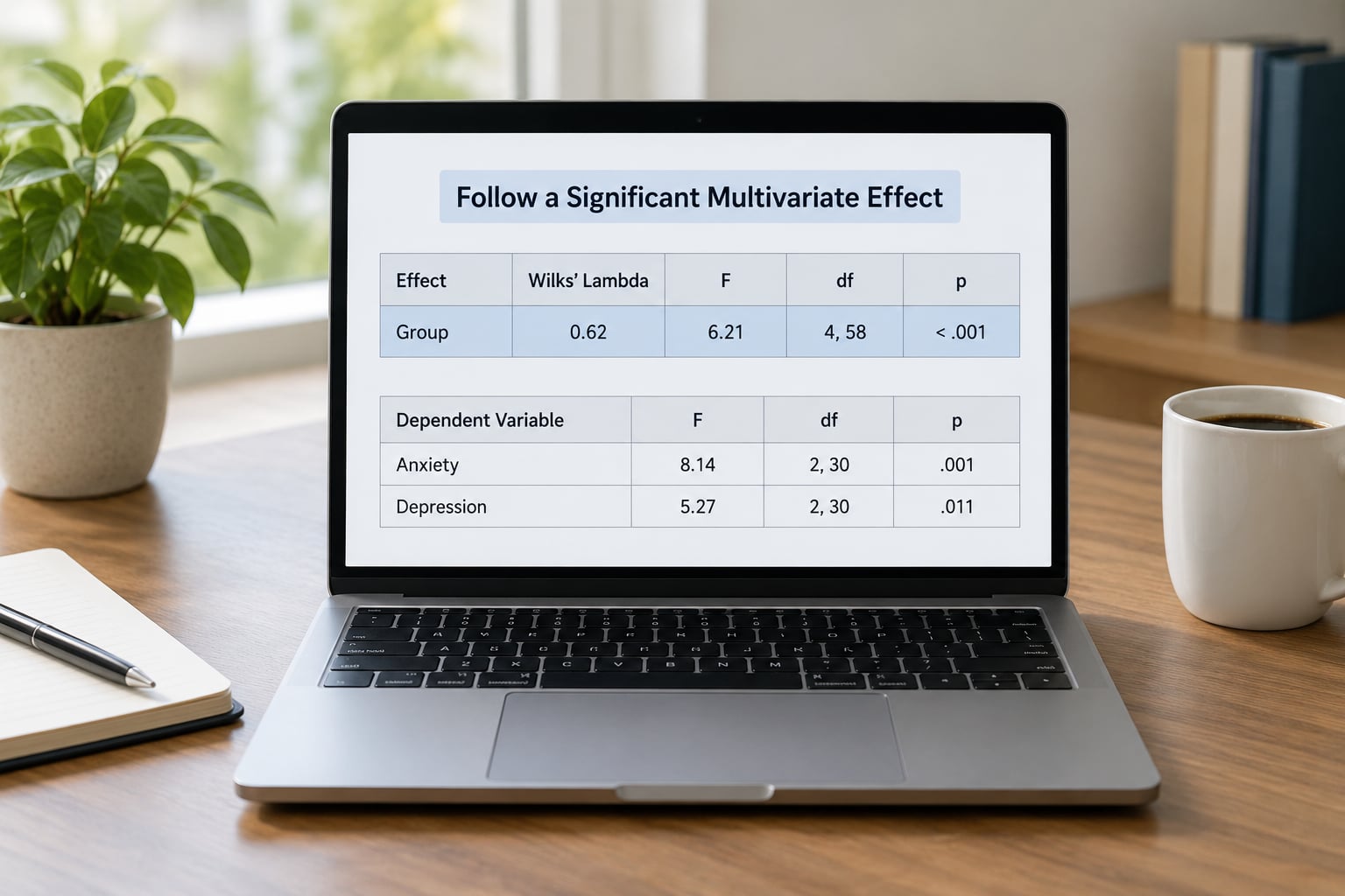
A significant Pillai’s Trace tells you that something differs. It does not tell you on which dependent variable, so you have to look next in the Tests of Between-Subjects Effects table. That table runs one univariate test per dependent variable and gives you the answer you actually need.

Reading the columns in order: Type III Sum of Squares is the variation explained by the model, df are the degrees of freedom, Mean Square is the sum of squares divided by df, F is the test statistic, Sig. is the p-value, and then the effect sizes sit at the right. Partial Eta Squared is the one to report for a factorial design, since it adjusts for the other effects in the model. R Squared (Eta Squared) is the unadjusted proportion of variance explained, useful as context but not the APA default when other terms are present.

Note that the tests in this table are unadjusted for the number of comparisons, so a significant multivariate result tells you to look, and the univariate rows tell you where. If you tested four dependent variables and all four are significant at .05, roughly one in five would be significant by chance alone, which is exactly the inflation MANOVA was designed to prevent.

Two situations confuse nearly everyone:

The omnibus is not significant but one dependent variable is very significant. This is the single most common forum question on this topic, and the answer is not that SPSS is broken. The omnibus test spreads the evidence across all outcomes, and one strong outcome cannot always carry the whole set. The omnibus test governs. You cannot claim a difference on a specific dependent variable when the multivariate test came back non-significant, and reporting the lone univariate result as if it were your finding is a genuine Type I error risk. Report the omnibus as non-significant and treat the design or sample as needing more data.

The omnibus is significant but the post hoc comparisons are not. This is normal and it usually reflects sampling error rather than a mistake. An omnibus test is more powerful than any single pairwise comparison, so it can detect a pattern that is too diffuse for one specific pair of groups to reach significance on its own. The UCLA SPSS Library makes this point directly: omnibus and pairwise tests can disagree, and it does not mean anything is broken.

For post hoc work, your choices are narrow and depend on design. Tukey is the standard for equal n and homogeneity, Games-Howell for equal variances violated with equal n, and Bonferroni or Sidak for unequal variances. If the factor has only two levels, no post hoc is needed at all, because the significant effect already identifies the two groups. If you have planned contrasts or theory-driven hypotheses, use those instead of a blanket post hoc, and say so in your methods.

Report and Visualize the Results

Write the result in APA 7 format, naming the test you chose. A filled example:

A multivariate analysis of variance was conducted to examine the effect of group membership on the combined set of test score and completion time. A significant effect of group membership was found on the combined dependent variables, Pillai’s trace = .184, F(2, 148) = 6.12, p < .001, partial eta squared = .076.

The fill-in-the-blank version, so you can adapt it:

A [significant / non-significant] effect of [factor] was found on the combined dependent variables, Pillai’s trace = [.000], F([hypothesis df], [error df]) = [.000], p [</=] [.000], partial eta squared = [.000].

For a two-factor design, report each main effect and the interaction separately, each with its own line. Follow the significant multivariate result with the relevant Tests of Between-Subjects Effects rows, then your post hoc or planned comparisons with their adjusted p-values and confidence intervals.

Do not cherry-pick. Running one univariate ANOVA per dependent variable after the fact and reporting only the ones that cross .05 without the omnibus is one of the most common reporting mistakes in student work, and it quietly undoes the error control you ran MANOVA for in the first place.

For visualization, a bar or line chart of the estimated marginal means per group is the standard companion figure. Plot the group means with an error bar, and keep dependent variables on separate charts unless you label the axes clearly. Estimated marginal means are preferable to raw means when you have covariates or unbalanced groups, because they adjust for the other terms in the model.

Common Mistakes

Almost every MANOVA mistake I see comes from one of these eight.

1. Putting the grouping variable into Dependent Variables. SPSS will run the analysis, and the result is meaningless. Fix: categorical variables go into Fixed Factors, always.
2. Running only one dependent variable. That is an ANOVA. MANOVA requires at least two continuous outcomes.
3. Treating a non-significant Box’s M as proof of normality. A non-significant result fails to reject the null; it does not confirm anything, especially with a small sample. Fix: check residual plots and Q-Q plots too.
4. Reporting only Wilks’ Lambda. Older tutorials push Wilks as the default. It is more vulnerable to non-orthogonal designs and unequal group sizes. Fix: report Pillai’s Trace.
5. Forgetting the interaction term in a two-factor design. SPSS builds only main effects by default. Fix: open the Model dialog and add the interaction before clicking OK.
6. Running unplanned post hoc tests after seeing the omnibus result. Selecting comparisons because they came out significant inflates Type I error. Fix: define comparisons in advance, or use an omnibus-protected approach and say what you did.
7. Reporting significance with no effect size. Sig. = .001 with partial eta squared of .01 is a very small effect in a big sample. Fix: always report partial eta squared alongside the p-value.
8. Ignoring the residual and outlier diagnostics. A single influential case can produce a significant MANOVA on its own. Fix: tick Residuals in Options and inspect the output.

Two more reporting habits worth building. Say in your methods section which test statistic you chose and why, so the choice is not an afterthought for your reader. And keep your syntax file. A short block of GLM Multivariate syntax in an appendix makes your analysis reproducible, which increasingly matters in thesis review.

Frequently Asked Questions

Conclusion

Start by putting your continuous outcomes in the Dependent Variables box and your categorical groups in Fixed Factors, then run Analyze > General Linear Model > Multivariate. That single dialog handles one-factor, two-factor, and repeated-measures designs, so the menu you need is already open in front of you.

Before you interpret anything, look at Box’s M, Levene’s test, the residual plots, and your group sizes. Then read Pillai’s Trace in the Multivariate Tests table, move to the Tests of Between-Subjects Effects to find which outcomes carry the effect, and report the result with the degrees of freedom, the exact p-value, and partial eta squared attached.