
To run logistic regression in SPSS, open your data file, go to Analyze > Regression > Binary Logistic, drop your 0/1 outcome into the Dependent box and your predictors into the Covariates box, then click OK. The whole run takes about two minutes. The part that takes longer is reading the output afterwards.
Logistic regression predicts the probability of a categorical outcome, usually a yes/no or pass/fail result, from one or more predictors. Unlike linear regression, it never predicts a value outside 0 and 1, and it reports its results as odds ratios rather than raw units. Here is the full walkthrough, including the menu route, the matching syntax, and how to read each output table without over-claiming anything.
Table of Contents
- 1What You Need
- 2Step-by-Step: How to Run Logistic Regression in SPSS
- 3Check Your Data and Variable Coding
- 4Open the Logistic Regression Dialog
- 5Select Predictors and Model Options
- 6Run the Analysis and Read the Model Summary
- 7Interpret Coefficients and Odds Ratios
- 8Check Classification and Goodness of Fit
- 9Test the Final Model and Residuals
- 10Report Your Logistic Regression Results
- 11Common Mistakes
- 12Frequently Asked Questions
- 13What are the assumptions of binary logistic regression?
- 14How do I interpret logistic regression output in SPSS?
- 15How do I find the odds ratio in SPSS?
- 16What does an odds ratio of 1.5 mean?
- 17Why did SPSS drop my cases in logistic regression?
- 18How do I add an interaction effect in SPSS logistic regression?
- 19Conclusion
What You Need
Four things have to be in place before you open the dialog, and every one of them saves you a confusing run later.
- A binary dependent variable coded 0 and 1. SPSS treats the outcome as the event being predicted, so 1 means the event happened.
- At least one predictor, numeric or categorical. Continuous variables like age or income go in as they are.
- Categorical predictors declared properly. A grouping variable with three or more levels cannot be entered as a plain covariate; it needs dummy coding through the Categorical button.
- A clean dataset with no impossible values and no missing data sitting in the outcome column.
Missing values are the quiet reason many first runs come back with a smaller N than expected. Before you start, run Analyze > Descriptive Statistics > Frequencies, tick Display frequency tables, and look at each variable you plan to use. Cases with a blank on any model variable get excluded, and SPSS reports the count in the Case Processing Summary.
You also need a version of IBM SPSS Statistics with the Analyze and Regression menus available. The menu names differ slightly between the subscription and academic licences, but the Binary Logistic dialog itself is identical. Screenshots in most tutorials come from older Windows builds, so if your dialog looks different, trust the box names rather than the layout.
Step-by-Step: How to Run Logistic Regression in SPSS
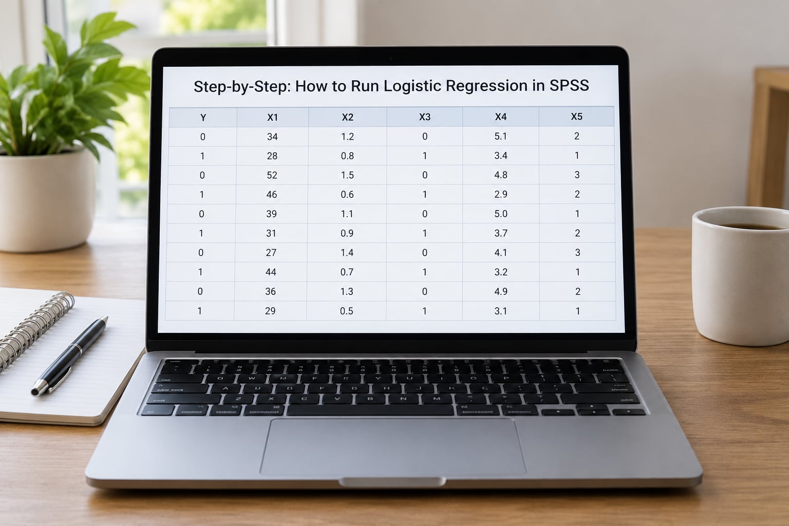
Check Your Data and Variable Coding
Open the Data View grid and look at your outcome column. If it holds 0s and 1s, you are ready. If it holds Yes and No, or 1 and 2, recode it first through Transform > Recode into Different Variables. Choosing the two categories carefully matters, because the group you set to 1 is the group every odds ratio refers back to.
Run Frequencies on the outcome to make sure it contains only the categories you expect, with no stray 9s, 99s or blanks acting as a hidden third category. Then check each predictor: a column that holds a handful of distinct labels is categorical, and a column with a wide spread of measurements is continuous.
Open the Logistic Regression Dialog
Go to Analyze > Regression > Binary Logistic. The dialog has five boxes on the left: Dependent, Covariates, Categorical, WLS Weight and Selection. Drop your 0/1 outcome into the Dependent box and your numeric predictors into Covariates.
Leave the Method dropdown on Enter. Enter puts every predictor into the model in one block and gives you the full Variables in the Equation table, which is what you want when your research question names specific predictors. Forward LR, Backward LR and Stepwise LR search for a subset, and they produce a different, less transparent table.
Select Predictors and Model Options
Move any grouping variable with more than two categories from Covariates to the Categorical box by clicking the arrow next to it. SPSS then opens the Categorical Variables Specification dialog, where you confirm the number of categories for each and can change the coding scheme.
The Reference category dropdown is set to First by default, meaning the first level listed is treated as the baseline and its coefficients are omitted. Choosing Last simply moves the baseline to the final category. Either is valid, but every coefficient in the output is measured against that baseline, so pick it deliberately and say which one you picked in your write-up.
Next open Options. Tick CI for exp(B) so you get confidence intervals for every odds ratio, and Hosmer-Lemeshow goodness of fit for a calibration check. Add Classification plot if you want a visual of predicted probabilities by observed group. Leave Iteration history off unless the model fails to converge and you need to see what happened. The Save sub-menu is where you can write predicted probabilities, predicted group membership, standardised residuals and Cook’s distance to new columns in your data file for later inspection.
Run the Analysis and Read the Model Summary
Click OK. SPSS runs the model and opens a Viewer window with the output. The same run in syntax looks like this:
LOGISTIC REGRESSION VARIABLES pass
  /METHOD=ENTER hours_studied attendance prior_gpa
  /CRITERIA=PIN(.05) POUT(.10) ITERATE(20)
  /PRINT=CI(95) HL
  /CLASSIFICATION
  /SAVE PREDPROB PRED GROUP RESID.
In the Model Summary table, read the Omnibus Tests of Model Coefficients row first. If Sig. is below .05, your predictors collectively improve on the intercept-only model, and the rest of the table is worth reading. A Sig. above .05 means the block adds nothing, and you should look at your model specification before interpreting individual coefficients.
Then compare the Cox and Snell R Square and Nagelkerke R Square values with the -2 Log Likelihood column. These are pseudo R-squared values, not the R-squared from linear regression. Cox and Snell never reaches 1, while Nagelkerke is rescaled so it can, which is why people usually report Nagelkerke.
If you are new to the output, this table is the shortest route through it. Read only the statistic in the third column and ignore the rest until you need it.
| Output table | What it tells you | The one statistic to read |
|---|---|---|
| Case Processing Summary | How many cases entered and why the rest were dropped | Valid and Excluded counts |
| Categorical Variables Coding | Which category became the baseline and how it was coded | The reference category row |
| Omnibus Tests of Model Coefficients | Whether the block improves on the intercept-only model | Sig. |
| Model Summary | Overall fit and the drop in -2 log likelihood | Nagelkerke R Square |
| Hosmer and Lemeshow Test | One calibration check on predicted probabilities | Sig., read with the large-sample caveat |
| Classification Table | How often predicted group matched observed group | Percentage Correct, Block 1 versus Block 0 |
| Variables in the Equation | The effect of each predictor on the odds | Exp(B) and its 95% confidence interval |
Interpret Coefficients and Odds Ratios
The Variables in the Equation table is the one most people open, and the columns that matter are B, the Wald statistic, Sig., Exp(B) and the 95% confidence interval for Exp(B). B is the change in log-odds per unit increase in the predictor. Exp(B) is that change expressed as a multiplier on the odds.
Here is a worked example. Suppose hours studied has a B of 0.85. Raise e to that number: e^0.85 is about 2.34. So each additional hour of study multiplies the odds of passing by roughly 2.3, holding attendance and prior GPA constant. The confidence interval is the part that tells you whether to write it up: if it runs from 1.9 to 2.9, the effect is precise; if it runs from 0.9 to 6.1, the estimate is too vague to say much about.
An Exp(B) of exactly 1.0 means no effect, and one below 1.0 means reduced odds. Because 1.5 means one and a half times the odds rather than 50% more likely, always check the Sig. column before describing anything.
Check Classification and Goodness of Fit
The Classification Table shows how often the model predicted the observed group. Read Percentage Correct in Observed Predicted, and remember that SPSS also prints the accuracy of the intercept-only model in Block 0. If Block 0 already classifies 80% correctly because your outcome is lopsided, a final accuracy of 82% tells you almost nothing.
Look at which group the model predicts. A Classification Table where every case lands in one column means the model has no discriminating power, even if the Omnibus test is significant. For a full picture you also want sensitivity and specificity, which you can build from the two off-diagonal counts.
The Hosmer and Lemeshow Test with Sig. above .05 is often quoted as proof of a good fit. It is not. The statistic is over-sensitive in very large samples, and a non-significant result on 15,000 cases can coexist with visibly poor calibration. Treat it as one piece of evidence, and pair it with a classification plot and a look at residuals.
Test the Final Model and Residuals
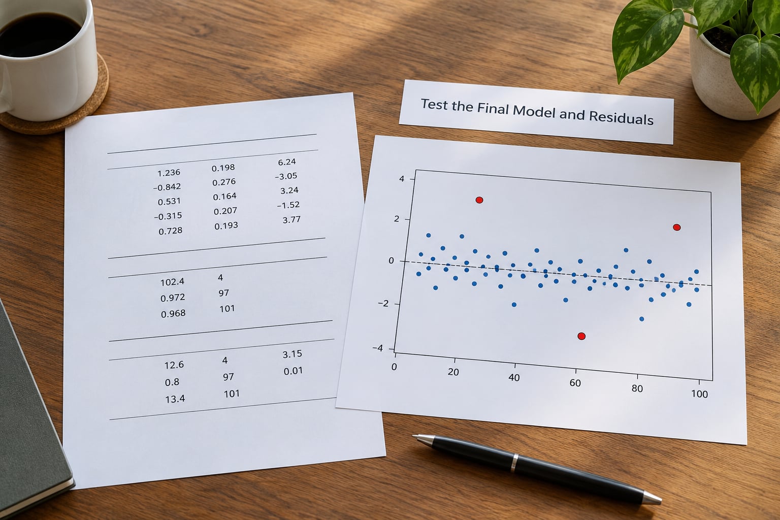
To test whether your predictors add explanatory power, run two models: one with the key predictor alone, then a second block adding the rest. The change in -2 log likelihood across blocks appears in the Omnibus Tests table as a Model Summary comparison, and that chi-square is the formal test. If you prefer the syntax route, use /METHOD=ENTER a b for the first block and /METHOD=ENTER a b c d for the full model, then compare the -2LL values by hand.
For influence, use the Save menu before you click OK. Add Cook’s distance and standardised residuals, run the model, then sort your data by Cook’s distance descending and inspect the top few cases. Anything above 1 deserves a look, and clustered high values signal cases the model fits badly. Check whether they are data errors, extreme outliers, or genuinely important cases that your model is missing.
Report Your Logistic Regression Results
APA reporting keeps to two sentences plus a table. Fill in the blanks:
A binary logistic regression examined whether [predictor] predicted [outcome]. The model was significant, chi-square(df = [ ]) = [ ], p = [ ], Nagelkerke R Square = [ ]. Holding [controls] constant, each unit increase in [predictor] multiplied the odds of [outcome] by [Exp(B)] (95% CI [ ]–[ ]), Wald([ ]) = [ ], p = [ ]. The model correctly classified [ ]% of cases.
Report every predictor you specified, including the non-significant ones. Dropping them from the write-up makes the model look stronger than it is. And keep the language careful: a significant odds ratio tells you the odds differ, not that the predictor causes the outcome.
Common Mistakes
Running binary logistic on three or more outcome categories. SPSS will refuse the analysis. For an ordered outcome such as poor, fair, good, use Analyze > Ordinal Regression (PLUM). For unordered categories with more than two levels, use Analyze > Generalized Linear Models > Multinomial (GENLIN). Dichotomising to force a binary model throws away information and needs a clear justification.
Coding the outcome as 1 and 2 instead of 0 and 1. SPSS accepts it and then reports odds in the wrong direction. Recode before running.
Leaving a categorical predictor in the Covariates box. SPSS treats the group labels as numbers, so the coefficient is meaningless and the Categorical Variables Coding table never appears. Move the variable into the Categorical box.
Reading a non-significant Hosmer-Lemeshow as perfect fit. It only means the test did not detect miscalibration at that sample size.
Overreading a pseudo R-squared. Values in the 0.2 range are common for real-world social science data, and no amount of added predictors reliably pushes a Nagelkerke value above about 0.5.
Ignoring influential cases. One case with a Cook’s distance above 1 can move a coefficient noticeably. Save the diagnostics and look.
Reporting odds ratios as probability changes. An odds ratio of 1.5 is not a 50% increase in probability. If you need probabilities, compute them from the model and report those separately.
Puzzled by the Case Processing Summary. The rows labelled Valid and Excluded show exactly how many cases were used and why the others were dropped, usually missing values or values outside the declared range.
Frequently Asked Questions
What are the assumptions of binary logistic regression?
The four checks that matter most are a genuinely binary outcome coded 0 and 1, independent observations, no perfect separation between predictors and outcome, and no severe multicollinearity among the predictors. You also want a reasonable number of outcome events, with roughly ten events per predictor as a common minimum guideline. Linearity in the logit matters for continuous predictors and can be checked by comparing the values of the continuous predictor against its mean logit.
How do I interpret logistic regression output in SPSS?
Start with the Omnibus Tests of Model Coefficients to confirm that your predictors collectively improve on the intercept-only model. Use the Model Summary for pseudo R-squared and the change in -2 log likelihood. Then read Variables in the Equation for B, the Wald test, Sig. and Exp(B) with its confidence interval. The Classification Table tells you how often predictions matched observed groups, and the Hosmer-Lemeshow test gives one calibration check.
How do I find the odds ratio in SPSS?
The odds ratio is already printed for you. In the Variables in the Equation table, the column labelled Exp(B) holds it, and it equals the base e raised to the power of B. Tick CI for exp(B) under the Options button before you run the model and SPSS also prints the lower and upper bounds of the 95% confidence interval in the two columns to the right.
What does an odds ratio of 1.5 mean?
An odds ratio of 1.5 means the odds of the outcome are one and a half times as high for that predictor, holding the other variables constant. It does not mean the outcome is 50% more likely. The difference matters most when the baseline probability is already high, because odds ratios exaggerate changes that look modest in probability terms.
Why did SPSS drop my cases in logistic regression?
Open the Case Processing Summary table at the top of the output. The Valid row tells you how many cases entered the analysis and the Excluded row gives the reason for each loss. The usual causes are missing values on the outcome or any predictor, and values outside the range you declared for a categorical variable. Filter the data file on missing values to find them quickly.
How do I add an interaction effect in SPSS logistic regression?
Use the Next button, written as u0026gt;a*bu0026gt; in the dialog, above the Covariates box. Select the two variables you want to interact and SPSS creates the product term as a new column in your data file. Add that new variable to the model and report the interaction first. Remember that you cannot add two odds ratios together; add the B coefficients and then exponentiate the sum.
Conclusion
Start by confirming your outcome is genuinely coded 0 and 1 with no stray codes hiding in it. Then run Analyze > Regression > Binary Logistic, declare your grouping variables through the Categorical button, tick CI for exp(B) under Options, and click OK. Read the Omnibus test, then the Model Summary, then the coefficients in Variables in the Equation. Report odds ratios with their confidence intervals and keep the claims to odds, not certainty about what happens next.