
The Durbin-Watson statistic is a number between 0 and 4 that measures whether consecutive residuals from a regression are related to each other. A value near 2 means no first-order autocorrelation, a value below 2 means positive autocorrelation, and a value above 2 means negative autocorrelation. Knowing how to interpret durbin watson statistic results comes down to judging distance from 2, then confirming what the plot and a formal test say.
Put the four numbers you need in front of you before you read anything else: the d value, your sample size n, the number of regressors k, and whether your rows are sorted in time order. If any of those is missing, the interpretation is guesswork.
- d close to 2.0 — residuals behave independently, nothing to correct.
- d between 0 and 2 — positive autocorrelation; below 1.5 is a cause for concern.
- d between 2 and 4 — negative autocorrelation; above 2.5 is a cause for concern.
- d between 1.5 and 2.5 — the widely quoted screen, which is a starting point and not a test.
Table of Contents
- 1What the Durbin Watson Statistic Measures
- 2How to Interpret Durbin Watson Statistic Values
- 3Durbin Watson Statistic Ranges at a Glance
- 4Why the Common 1.5 to 2.5 Rule Is Only a Guide
- 5How the Durbin Watson Statistic Is Calculated
- 6How to Check Autocorrelation After the Statistic
- 7What Different Durbin Watson Results Mean in Practice
- 8Sample Size and Model Specification Considerations
- 9How to Report the Result in a Thesis or Paper
- 10Frequently Asked Questions
- 11Is a Durbin Watson value of 1.9 always acceptable?
- 12Why is my Durbin Watson statistic greater than 2?
- 13Does the Durbin Watson test have a p-value?
- 14What Durbin Watson value is considered evidence of autocorrelation?
- 15Is the Durbin Watson test appropriate for logistic regression?
- 16Conclusion
What the Durbin Watson Statistic Measures
The Durbin-Watson statistic, published by James Durbin and Geoffrey Watson in 1950, tests one specific assumption: that the errors in an ordinary least squares model are not serially correlated. Serial correlation simply means that once an observation runs above its fitted value, the next observation tends to run above its fitted value too.
This is not the same problem as heteroscedasticity. Heteroscedasticity is residual spread that grows across the sample — a funnel shape on a residual-versus-fitted plot. Autocorrelation is residual spread that follows the order of your rows. Your data can be perfectly homoskedastic and still badly autocorrelated, and vice versa.
Understanding how to interpret durbin watson statistic output starts with knowing what the numerator and denominator are doing. The statistic compares how far each residual jumps from the one before it with how large the residuals are overall. When residuals leap about unpredictably from period to period, jumps are large and the ratio lands near 2. When residuals run in clusters above and below zero, jumps are small and the ratio drops below 2.
It is a first-order diagnostic. It looks at consecutive pairs only, so a pattern with structure at lag 3 or lag 4 can still produce a d near 2 while your residuals remain badly dependent.
How to Interpret Durbin Watson Statistic Values

Here is the short answer to the main query. A d value near 2 suggests no first-order autocorrelation. A value below 2 suggests positive autocorrelation, and a value above 2 suggests negative autocorrelation. The further the value sits from 2, the stronger the dependence between adjacent residuals.
What the statistic does not do is decide statistical significance. It carries no p-value on its own and cannot tell you whether your model is correctly specified. A d of 1.4 and a d of 1.6 look very different, but neither is automatically a problem: it depends on n, on k, and on the critical values for your design.
Two common misreadings are worth naming. Treating a value above 2 as a broken model is wrong; negative autocorrelation is unusual in economic time series but perfectly possible, and it inflates standard errors rather than shrinking them. The second is treating 2.0 as a magic target. The same model can return roughly 2.005 when you test two lags and roughly 1.95 when you test eight, two reassuring-looking numbers that say opposite things about the second and third lag.
Durbin Watson Statistic Ranges at a Glance
| d value | Interpretation | What to do next |
|---|---|---|
| Below 1.0 | Strong positive autocorrelation; residuals cluster in long runs | Treat the model as misspecified until proven otherwise. Re-estimate with GLS or heteroskedasticity-and-autocorrelation consistent standard errors. |
| 1.0 to 1.5 | Positive autocorrelation worth investigating | Check the residual time-order plot and run a Breusch-Godfrey test. |
| 1.5 to 2.5 | Screen says no concern | Confirm with the dL and dU values for your n and k. A screening guide is not a decision. |
| Exactly 2.0 | Adjacent residuals are about as different as random pairs | No correction needed on this ground. The test has told you nothing else. |
| 2.5 to 3.0 | Negative autocorrelation | Rare in economic data, common when residuals over-correct. Look for oversmoothing or differencing. |
| 3.0 to 4.0 | Strong negative autocorrelation; residuals alternate sign | Check for an over-differenced series or a model fitted to alternating data. |
These ranges are screening guides. They are not universal pass-or-fail thresholds, and they change with sample size and lag structure.
Why the Common 1.5 to 2.5 Rule Is Only a Guide
The 1.5 to 2.5 band comes from the sampling distribution of d under the null of zero first-order autocorrelation. For a large sample with many observations, that distribution concentrates near 2, so a band two-sided around the centre works reasonably well. Shrink the sample and the distribution flattens and spreads, and 1.5 to 2.5 stops being a safe screen.
Three things quietly break the rule. Sample size is the big one: with fewer than about 30 ordered observations the statistic is noisy. Lag structure is the second: if you have fitted a model with a lagged dependent variable, the standard Durbin-Watson is not valid at all. Residual ordering is the third, and it is the most common beginner error — run the test on rows sorted alphabetically or by an identifier instead of by date and the number is meaningless.
No cutoff can prove residuals are independent. Independence is a property of the data-generating process, and a statistic computed from finite data can only raise or lower your suspicion. A formal test gives you a p-value and a decision rule; a plot shows you the shape of the problem. Use both.
How the Durbin Watson Statistic Is Calculated
The formula is d = Σ(ut − ut−1)² / Σut², where ut is the residual for period t.
The denominator is the residual sum of squares: how far your points sit from the fitted line overall. The numerator is the sum of squared differences between adjacent residuals: how much each residual jumps relative to the one immediately before it. If residuals alternate wildly, the numerator is roughly twice the denominator and d approaches 2.
Here is a complete example. Take eight ordered residuals from a fitted model:
0.4, −0.2, 0.1, −0.3, 0.2, 0.3, −0.1, −0.4
| Step | Working | Result |
|---|---|---|
| Residual sum of squares | 0.16 + 0.04 + 0.01 + 0.09 + 0.04 + 0.09 + 0.01 + 0.16 | 0.60 |
| Squared changes between adjacent residuals | 0.36 + 0.09 + 0.16 + 0.25 + 0.01 + 0.16 + 0.09 | 1.12 |
| d statistic | 1.12 / 0.60 | 1.87 |
A d of 1.87 sits comfortably inside the screening band. Notice the residuals here are not random-looking — there are two positive runs and a negative one — yet the single statistic stays near 2. That is the clearest argument for looking at the residual plot as well.
There is also a useful shortcut. The statistic is roughly d ≈ 2(1 − r1), where r1 is the sample autocorrelation of the residuals at lag 1. That relationship lets you predict the answer: residuals with r1 of 0.2 give a d near 1.6, and residuals with r1 of −0.3 give a d near 2.6.
How to Check Autocorrelation After the Statistic
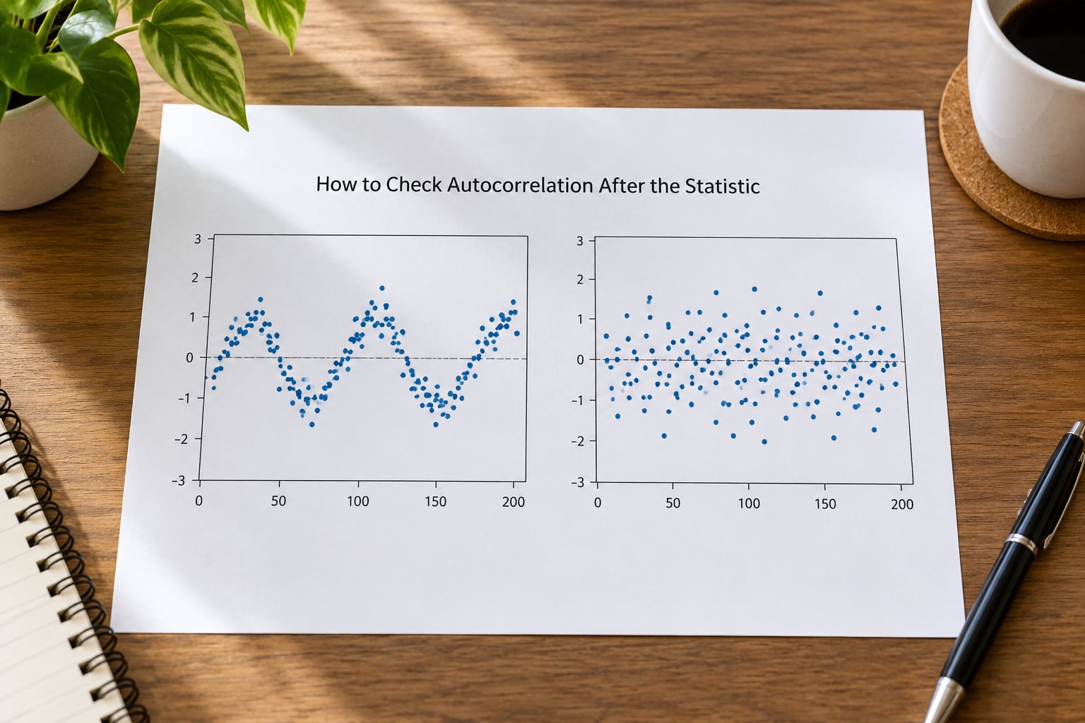
Most packages print the number and stop there. The habit worth building is to treat that number as the start of a diagnostic sequence rather than the end of one.
- Confirm the row order. Sort by time, by wave number, or by whatever the natural sequence is, then re-run. If your d moves a lot after sorting, your original value was an artefact of the ordering.
- Plot residuals in sequence order. Smooth waves or long same-sign stretches mean positive autocorrelation. Strict alternation means negative autocorrelation.
- Plot residuals against fitted values. A random cloud is what you want. A funnel there is heteroscedasticity, a separate problem that the Durbin-Watson statistic cannot see.
- Count runs of same-sign residuals. A long run of positives or negatives is direct evidence that adjacent residuals are linked.
- Run a formal test when the decision matters. Breusch-Godfrey, also called Cumby-Huizinga, tests several lags at once. Ljung-Box on the residual autocorrelation function works well when you want a single number for the whole pattern.
If a researcher wants a defensible sentence in a paper, that sequence is where it comes from. Learning how to interpret durbin watson statistic results is mostly about not stopping at the number your software printed under “Model Summary”.
What Different Durbin Watson Results Mean in Practice
A d near 0. Residuals are almost copies of their predecessors. Something systematic is left in the residuals, most often a missing time trend or an omitted variable that moves slowly across the sample.
A d near 1. Clearly positive dependence, roughly r1 of 0.5. Standard errors are too small, t-statistics too large, and any effect you declared significant deserves a second look.
A d near 1.5. Mild positive autocorrelation sitting just under the screening band. Do not rebuild the model over this. Look at the residual plot and run Breusch-Godfrey at two or three lags.
A d near 2. Little first-order linear dependence. Say so plainly and move on to other diagnostics, because a comfortable d says nothing about linearity, normality, or heteroscedasticity.
A d near 2.5. Mild negative autocorrelation. It usually appears when a model has absorbed an alternating pattern it should have modelled directly, or when a series has been differenced twice when once was enough.
A d near 3. Strong alternation between adjacent residuals. Check for over-differencing, or for a specification that forces an unrealistic zigzag.
A d near 4. Residuals flip sign almost every period, which points to a wrongly ordered or wrongly coded series, or to a first difference applied to data that was already stationary.
Extreme values can also come from specification problems rather than the residual process itself: a missing time trend, clustered observations from repeated measures on the same units, or rows left in an arbitrary order.
Sample Size and Model Specification Considerations
Sample size changes how much weight the number deserves. In a small sample the statistic is unstable, and the formal dL and dU decision rules were designed for exactly this situation: you look up two critical values for your n and k, and you compare rather than eyeball.
Lagged dependent variables are the case to know. The Durbin-Watson statistic assumes strictly exogenous regressors, and a lagged dependent variable is not exogenous — it is built from the same residuals you are testing. The statistic is only valid when every regressor is strictly exogenous, so it is not appropriate when a lagged dependent variable sits on the right-hand side. Use Breusch-Godfrey, Durbin’s h, or a lagged-residual t-test instead.
Repeated and clustered observations raise a different issue. With several measurements per unit, residuals within a cluster are correlated by construction, and a global d conflates that structure with genuine time dependence. Mixed-effects models or cluster-robust standard errors handle it better.
Missing values cause trouble in an unexpected way. If your software dropped rows with gaps, the surviving rows may no longer be evenly spaced, and the “consecutive” residuals in the formula are no longer consecutive periods.
When dependence is real and you need corrected coefficients rather than corrected standard errors, generalized least squares is the principled route. When you mainly need honest inference on coefficients you already trust, Newey-West standard errors do the job with far less work. Cochrane-Orcutt transformation is a middle path that re-estimates the model iteratively.
How to Report the Result in a Thesis or Paper
Report the statistic, the decision basis, and the conclusion — in that order, and nothing more than the evidence supports. The table below contrasts wording that overreaches with wording that holds up.
| Weak | Acceptable |
|---|---|
| The Durbin-Watson value is 1.98, so there is no autocorrelation. | The Durbin-Watson statistic was 1.98, indicating no evidence of first-order autocorrelation in the residuals. |
| The test proved the residuals are independent. | No evidence of first-order autocorrelation was detected at the 5% level, d = 1.98. |
| DW = 0.84, so the model is bad. | The statistic of 0.84 falls below the lower critical value, so first-order positive autocorrelation cannot be ruled out; the model was re-estimated using generalized least squares. |
| The p-value for the Durbin-Watson test was 0.03. | Using the Breusch-Godfrey test at two lags, serial correlation was present, p < .05; the Durbin-Watson statistic is reported descriptively because the model contains lagged dependent variables. |
When you do report formally, compare d with the dL and dU values from a Durbin-Watson significance table for your n, k, and significance level. If d is below dL, reject the null of no positive autocorrelation. If d is above dU, do not reject. If d falls between dL and dU, the test is inconclusive. For negative autocorrelation, run the same comparison on 4 − d.
A worked case from the standard literature makes this concrete. With n = 15, k = 1 at the 5% level, the table gives dL = 1.077 and dU = 1.361. A computed d of 1.89 sits above dU, so the null of no positive autocorrelation is not rejected. The same run with 4 − d = 2.11 would also fall outside the inconclusive band on the upper side, so negative autocorrelation is not indicated either.
Frequently Asked Questions
Is a Durbin Watson value of 1.9 always acceptable?
Usually, yes, but a single number never settles the question. A d of 1.9 falls inside the 1.5 to 2.5 screening band and is close to 2.0, so first-order dependence is weak. To be sure, compare it with the dL and dU values for your sample size and number of regressors, then look at the residuals plotted in time order. A value near 2 can still hide structure at lags beyond 1.
Why is my Durbin Watson statistic greater than 2?
A value above 2 means adjacent residuals tend to have opposite signs, which is negative autocorrelation. It is common in over-differenced series and in models fitted to data that alternates. It is rarer in economic time series than positive autocorrelation, so check that your rows are in the correct order and that you have not differenced a series twice. The formal test for it is the same dL and dU comparison applied to 4 minus d.
Does the Durbin Watson test have a p-value?
Not in its classical form. It uses two critical values, dL and dU, taken from a significance table rather than a single p-value. Because the exact distribution depends on sample size and lag structure, some software reports an approximate p-value alongside the statistic. Treat any such number as a convenience, and prefer the Breusch-Godfrey test when your model contains lagged dependent variables, since the classical Durbin-Watson is not valid there.
What Durbin Watson value is considered evidence of autocorrelation?
There is no single cutoff, which is the honest answer. As a screen, values below 1.5 or above 2.5 are treated as a cause for concern. As a formal decision, evidence depends on where your value falls relative to dL and dU for your sample size and number of regressors. A formal test with several lags, such as Breusch-Godfrey, gives a firmer answer because it can detect structure the single-pair statistic cannot.
Is the Durbin Watson test appropriate for logistic regression?
Not directly. It is built for continuous residuals from a linear model, and logistic regression produces bounded, non-normal residuals for which the test has no exact distribution. Check for dependence among the events in your ordered data instead, and handle it with a model that accounts for clustering, such as a mixed-effects logistic model or generalized estimating equations. If you also fitted a linear model to the same data, the Durbin-Watson statistic is still a valid check there.
Conclusion
The decision rule in one sentence: measure the distance between your d value and 2, then confirm with residual diagnostics or a formal test before you change anything.
Find the Durbin-Watson value in your model output, check how far it sits from 2 and in which direction, and look up dL and dU for your sample size and number of regressors. If your model contains lagged dependent variables, skip the statistic entirely and run Breusch-Godfrey instead. Working through how to interpret durbin watson statistic results is quick work once the sequence is a habit.