How to Run Exploratory Factor Analysis in SPSS (October 2026)

To know how to run exploratory factor analysis in SPSS, open your data file, go to Analyze > Dimension Reduction > Factor, move your scale items into the Variables box, tick the statistics you need under Descriptives and Extraction, pick a rotation, and press OK. The whole thing takes about ten minutes once your data are clean.

That menu path is the whole answer, but the clicking is the easy half. Most of the trouble people hit comes from putting the wrong variables in the box, leaving SPSS on its principal components default, and then reporting a solution that the loadings do not support. This guide walks through the dialog box button by button, then tells you how to read what comes out.

Here is the short version of the workflow:

1. Check your data are suitable: enough cases, correlated items, no demographics in the box.
2. Open Analyze > Dimension Reduction > Factor.
3. On Descriptives, request correlations, KMO and Bartlett’s test of sphericity.
4. On Extraction, choose principal axis factoring and keep the scree plot.
5. On Rotation, choose varimax first, then check factor correlations and switch to oblimin if needed.
6. Read communalities, total variance explained and the rotated matrix before you name anything.

Written and updated for 2026. The steps below match the IBM SPSS Statistics desktop interface (Windows and macOS menus are the same; the labels on some older releases read slightly differently).

Table of Contents

1. 1What You Need
2. 2Items as variables, not cases
3. 3Measurement level
4. 4Enough cases
5. 5Correlated items, and nothing pathological
6. 6Missing values, sorted out in advance
7. 7Exploratory, not confirmatory
8. 8Step-by-Step
9. 91. Prepare and Check Your Data
10. 102. Open the SPSS Factors Dialog Box
11. 113. Select the Extraction Method
12. 124. Choose and Interpret the Rotation Method
13. 135. Request the Necessary Output
14. 146. Interpret the Factor Solution and Write the Results
15. 15Common Mistakes
16. 16Frequently Asked Questions
17. 17What is the difference between EFA and CFA?
18. 18What is the minimum sample size required for exploratory factor analysis?
19. 19What is a scree plot in factor analysis?
20. 20What is varimax rotation in factor analysis?
21. 21What does cross-loading mean in factor analysis?
22. 22What is a good factor loading score in SPSS?
23. 23Conclusion

What You Need

You need IBM SPSS Statistics, a saved data file, and a dataset structured so that each survey item is a separate variable and each respondent is a separate case. If your items are sitting as columns B through Z of a spreadsheet, save that sheet as a .sav file first and open it in SPSS.

Items as variables, not cases

Factor analysis reads the correlation matrix between variables, so it needs items in the variable direction. One row per participant, one column per item. Age, gender, education level and other demographics stay out of the Variables box entirely; they are not indicators of a latent construct and they will distort the solution.

Measurement level

Continuous or scale variables work. Likert items coded 1 to 5 or 1 to 7 work, which is the normal case for most survey instruments. Nominal categorical variables (a yes/no item, a single-choice item, a dummy variable) should not go in as factor indicators: the arithmetic on their correlations is not meaningful. Dichotomous items can be handled in a separate treatment, but that is a different conversation.

Enough cases

The common rule of thumb is 5 to 10 cases per variable, and Tabachnick and Fidell treat that as the floor, not the target. Comrey and Lee give a harsher scale: below 50 cases very poor, 100 poor, 200 fair, 300 good, 500 very good. Students who end up at the low end usually have a marginal variable count and an ambitious scale, so the fix is more cases or fewer items.

Correlated items, and nothing pathological

Items in the same scale should correlate with each other, and the whole set must form a factorable matrix. You will see this formally in the next section. For now, the rule of thumb is that some correlation structure must exist. If your items are all near zero with each other, no factor analysis will help.

Missing values, sorted out in advance

SPSS deletes cases listwise by default, which means a participant missing any one item drops out of the entire analysis. That quietly shrinks N between your first and second runs. Check the extent of missingness with Analyze > Descriptive Statistics > Frequencies before you start, and if you want a different treatment, the Options dialog lets you switch to pairwise or exclude listwise.

Exploratory, not confirmatory

EFA is for when the structure is unknown and you want the data to tell you. Confirmatory factor analysis is for when you have a specified model and want to test it. Running CFA on the same data you used to discover the structure gives you artificially good fit, and most examiners will ask about that. The first entry in the FAQ below covers the difference in short form.

Step-by-Step

This is the full click path for how to run exploratory factor analysis in SPSS, with what each dialog button does and how to tell it worked.

1. Prepare and Check Your Data

Open the file and run Analyze > Descriptive Statistics > Frequencies on your items. Confirm each is numeric, check the minimum and maximum match your coding scheme, and look at how many cases are lost to missing data. A common surprise is an item imported as text, which SPSS silently treats as invalid and quietly excludes.

Then look at the correlation structure before you factor anything. Run Analyze > Correlate > Bivariate with your items, and scan for three things: the diagonals are 1.00, the off-diagonal correlations have a meaningful sign pattern, and no item correlates near perfectly (above about .90) with another, which usually means duplicate wording.

Decide the scope of the analysis here too, because it is the question students ask most often. If your instrument holds several distinct scales, run one analysis per scale. Pool every item from every scale into one run and the analysis will still return something, but it will mix your measurement model with your data reduction goal and produce a solution that reads oddly in Chapter 4.

One caution on nominal items: do not include demographics such as age, gender or job role as factor indicators. If you want to know whether they relate to the factors, compute factor scores first, then compare group means.

2. Open the SPSS Factors Dialog Box

Go to Analyze > Dimension Reduction > Factor. The dialog box has an Available Variables list on the left and a Variables box on the right.

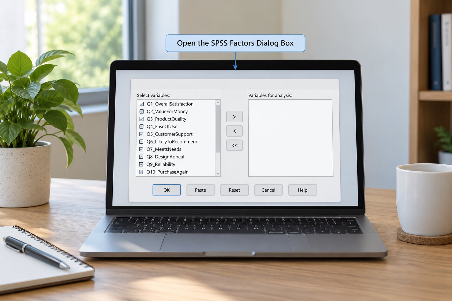
Move only the items you intend to factor into the Variables box. On the right is Extraction, which tells SPSS how many factors to keep, and below it Rotation, which decides how the solution is arranged for interpretation. Statistics and Options open two further dialogs. Before you press OK, check the dialog that is current.

You can do the whole thing from syntax instead, which is faster once you have run it a few times. A working version is at the end of this section.

3. Select the Extraction Method

Click Statistics, then Descriptives. Tick Correlations, KMO and Bartlett’s test of sphericity and Anti-image diagonal. These three give you the sampling adequacy and sphericity checks. If you also want the raw correlation matrix in the output, tick Coefficients, which is usually worth it in a thesis appendix.

The Kaiser-Meyer-Olkin measure reports sampling adequacy on a 0 to 1 scale. Above .80 is good, .60 to .79 is acceptable, .50 to .59 is marginal and below .50 means the correlation matrix is not factorable as it stands. Bartlett’s test of sphericity should come out significant at p < .05; a non-significant result means the correlation matrix is an identity matrix and factor analysis is inappropriate.

For the anti-image matrix, look at the diagonal of the anti-image correlations (partial correlations). Values below about .50 are poor, and those variables are the ones dragging your KMO down.

Then click Extraction. The dialog opens on Principal components, which is the SPSS default and not what most methodology sections want you to report. Choose Principal axis factoring for latent trait work on Likert scales, because it estimates common factor variance and is the standard in most social science methodology guides.

Method	What it estimates	Use it when
Principal components analysis	Total variance, including unique and error variance	You want maximum data reduction, or prediction rather than latent traits
Principal axis factoring	Common (shared) variance only	Scale and trait research on survey items, which is most theses
Maximum likelihood	Common variance with standard errors and fit tests	You want inferential statistics on the solution, or mixed item types

Keep Analyze set to Correlation matrix for Likert items and smaller samples. Correlation matrix works on standardized data and keeps communalities on a comparable 0 to 1 scale. Covariance matrix makes sense only if your items are on genuinely different scales and you care about the unstandardized solution.

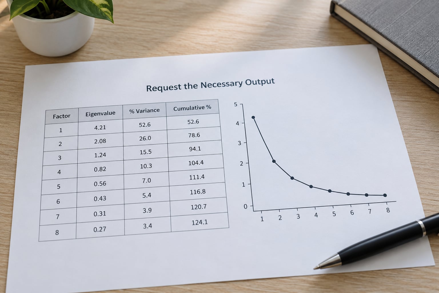
Leave Maximum iterations at 25 unless it fails to converge. Tick Display unrotated factor solution and Display scree plot. The scree plot is the graph of eigenvalues by component number, and the elbow, where the curve flattens out, is your evidence for how many factors to keep. The eigenvalue-greater-than-one rule is a rough starting point; the elbow and parallel analysis usually agree with it more closely.

Requesting KMO and Bartlett’s test inside the Extraction box instead puts those results right above the communalities table, which many people find easier to find later.

4. Choose and Interpret the Rotation Method

Rotation does not change the factor solution, only the coordinate system used to display it. Without rotation you usually get one dominant factor that loads on everything and a set of tiny factors that load on single items, which is unreadable.

Click Rotation. Varimax is preselected. It is an orthogonal rotation, which forces the factors to be uncorrelated, and it delivers the simplest structure, where each item loads clearly on one factor. That is the right first move for most instruments.

If your theory says the factors should be related to each other, or you suspect they are, use an oblique rotation instead: Direct Oblimin with delta set to 0 (SPSS default) or a small value like .5, or Promax with a power value of 4 or 5. Oblique rotation is usually more accurate when factors correlate, and it is the more defensible choice for most personality and attitude scales.

Rotation	Type	Factor correlations	Choose it when
Varimax with Kaiser normalization	Orthogonal	Forced to zero	You want clean simple structure and expect independent dimensions
Direct Oblimin	Oblique	Estimated from data	Factors probably relate; most flexible option
Promax	Oblique	Estimated from data	Many correlated factors, large item sets

How do you tell which you need? Run varimax first, then scroll to the Component Correlation Matrix at the end of the output. If the off-diagonal correlations are near zero, varimax was fine. If several are .30 or above, re-run with oblimin or promax and report that instead.

5. Request the Necessary Output

Click Options. Under Missing values, listwise is the default and matches what most textbooks assume. Tick Display sorted by size so loadings appear in descending order inside each factor block, which makes the structure far easier to read. Tick Suppress small loadings and set the value to .30 if you want SPSS to blank out anything below that, but do not set it too high or you will hide loadings you need to argue about. K iterations only applies to promax and oblimin; leave it at 25.

Tick Rotate factor solution here rather than on the Rotation tab if you would rather see the unrotated solution first, which is useful for confirming simple structure before rotation reshapes it.

Now press OK. The output viewer produces, in this order: the Statistics table (correlations, KMO, Bartlett’s), the Communalities table, the Total Variance Explained table, the scree plot, the unrotated solution if requested, the rotated component matrix, the component plot and plot of rotated solutions, the factor transformation matrix, the component correlation matrix if you rotated obliquely, and the factor score coefficient matrix.

6. Interpret the Factor Solution and Write the Results

Read the output in this order, because each table depends on the last one. Most walkthroughs of how to run exploratory factor analysis in SPSS stop once they reach the rotated matrix, which is exactly the table you should not stop at.

KMO and Bartlett’s. KMO above .60 and Bartlett’s p < .05 mean the matrix is factorable. Anything less and you should stop and fix the item set before reading anything else.

Communalities. This is how much variance in each item is shared with the other items. Initial communalities are 1.00 for every item. Extraction communalities below .40 mean the item is poorly explained by the solution, and below .30 usually means it does not belong. Multiple regression instead of common factor analysis will inflate these values, so compare cautiously if you used PCA.

Total Variance Explained. Eigenvalue, percent of variance, and cumulative percent. This is where you fix your factor count. Count the components with eigenvalues above 1, then check the scree plot elbow, then consider parallel analysis for an objective comparison.

Rotated Component Matrix. The heart of the analysis. Each number is a factor loading, and the size tells you how strongly an item belongs to a factor.

Loading size	Reading	What to do
.70 and above	Strong, the item defines the factor	Keep it, it is your clearest marker
.50 to .69	Good	Keep it
.40 to .49	Acceptable, the usual floor	Keep it and check for cross-loading
.32 to .39	Weak	Consider removal if theory allows it
Below .32	Poor	Drop the item and re-run

High loadings mean the item shares most of its variance with that factor, so it is measuring what that factor represents. A .75 loading means roughly 56% of the item’s variance sits on the factor. Loading strength scales differ slightly by field, and the .32 and .45 cut-offs you see in older texts refer to a criterion where the cross-loading on another factor must be lower still.

Cross-loadings. An item that loads .45 on one factor and .42 on another is ambiguous, and you need to resolve it rather than hope nobody reads the table. The practical rule: if the primary loading is at least .10 higher than the next highest, keep the item; if the difference is under .10, delete it and re-run. Deleting items one at a time and re-running each time, rather than deleting a batch, avoids removing more than you need.

Naming the factors. Name each factor after its highest-loading items, not after your hypothesis. Use plain descriptive language, note which items mapped to which factor, and avoid anything causal. A factor named “Job Satisfaction” is a label for a pattern of responses; it does not cause, mediate or predict anything.

Here is the full syntax if you prefer the command window. Paste it, swap your variable names in, and run it:

FACTOR
  /VARIABLES q1 q2 q3 q4 q5 q6 q7 q8 q9 q10 q11 q12
  /MISSING LISTWISE
  /ANALYSIS q1 q2 q3 q4 q5 q6 q7 q8 q9 q10 q11 q12
  /PRINT INITIAL KMO EXTRACTION ROTATION
  /FORMAT SORT BLANK(.30)
  /CRITERIA FACTORS(4) ITERATE(25)
  /EXTRACTION PAF
  /CRITERIA ITERATE(25)
  /ROTATION VARIMAX
  /METHOD=CORRELATION.

To go oblique, change /ROTATION VARIMAX to /ROTATION OBLIMIN or /ROTATION PROMAX(4). To save factor scores as new variables, append /SAVE REG(ALL), then use those variables as your sub-scale scores, and run Analyze > Scale > Reliability Analysis for Cronbach’s alpha on each factor’s items.

Common Mistakes

These are the errors that show up again and again, and each has a fix.

Everything goes into the Variables box. Demographics, open-text coded variables, an item on a different construct. Check the list one item at a time before you run it, and if your instrument has separate scales, factor each one separately.

Leaving principal components as the default. SPSS opens the Extraction dialog on PCA and many students never touch it. If your methodology chapter specifies principal axis factoring, switch it and report what you actually ran.

Varimax when your factors clearly correlate. Check the Component Correlation Matrix at the end of the output. Off-diagonal values of .30 or more mean you need an oblique solution.

Ignoring cross-loadings. An item loading .40 on two factors is not a result, it is an unresolved item. Decide it explicitly and say what you did in the write-up.

Choosing the factor count from eigenvalues alone. The eigenvalue-greater-than-one rule tends to over-retain with small item counts. Use the scree plot elbow alongside it, and parallel analysis if you can get your hands on a random-data comparison.

Treating a factor label as a causal claim. Factor analysis describes variance structure in your sample. It does not explain why the items correlate.

Reporting without the details. Your methods section needs the N actually used after listwise deletion, the extraction method, the rotation and its parameters, the missing-data treatment, the number of items, and the variance explained. Examiners ask for all of it.

A short quality-control pass before you write: KMO above .60, Bartlett’s significant, no communality under .40, most loadings at .50 or above, no unexplained cross-loading, and a scree plot whose elbow matches your retained solution. Fix what fails and re-run rather than writing around it.

Frequently Asked Questions

Conclusion

Start by confirming your data are factorable: enough cases, correlated items, no demographics in the box. Run the analysis from Analyze > Dimension Reduction > Factor with principal axis factoring and varimax, then read KMO, Bartlett’s, communalities, the scree plot and the rotated matrix in that order.

If the factors correlate, re-run with oblimin or promax. Resolve cross-loadings one item at a time, re-run, and compute Cronbach’s alpha for each resulting sub-scale. Finally, record your N, extraction method, rotation and missing-data treatment so your methods section matches your output exactly. That is how to run exploratory factor analysis in SPSS and end up with a solution you can defend.