How to Run a One Sample t Test and Report It in SPSS 2026

A one-sample t-test asks one simple question: is the mean of my sample meaningfully different from a value I already know? To learn how to run a one sample t test and report it in SPSS, put your continuous measure in the Test Variable box, type the benchmark into Test Value, then read the t, df and Sig. (2-tailed) columns out of the One-Sample Test table and write them up in APA format. It takes about ten minutes once your data is clean.

I have watched students run this test correctly and then report p = .000 because SPSS printed three zeros. That single formatting slip is the most common problem in the whole procedure, and it is easy to avoid once you know where it comes from.

Table of Contents

1. 1What You Need
2. 2Step-by-Step: How to Run a One Sample t Test and Report It
3. 31. Prepare the Variable and Data
4. 42. Check the Assumptions
5. 53. Enter the Test Value
6. 64. Run the Test in SPSS
7. 75. Interpret the Output
8. 86. Report the Result in APA Style
9. 9Common Mistakes
10. 10Practical Tips and Reporting Checklist
11. 11Frequently Asked Questions
12. 12How do I run a one sample t-test in SPSS?
13. 13Why does SPSS print Sig. (2-tailed) = .000?
14. 14What assumptions do I need to check first?
15. 15When should I use a one-tailed test instead?
16. 16How do I interpret a non-significant result?
17. 17How do I report the result of a paired or independent samples t-test?
18. 18Conclusion

What You Need

Before you open SPSS, sort out four things. The test is meaningless without them, and each one takes longer to fix later.

• One continuous dependent variable. It must be measured at interval or ratio level, which rules out categories like course grade or yes/no answers.
• A defensible test value. This is the number your sample is being compared against: a published population mean, a national average, a clinical cutoff, an exam pass mark. It has to come from a source, not from your own data.
• Clean data. No text in the variable column, no stray codes, and a decision about missing values made in advance.
• An alpha level. .05 is the default and the one you should report. Choose it before you see the output, not after.

Sample size matters less than people think. The test works fine below 30 cases; it just leans harder on the normality assumption as n shrinks, which is why checking a boxplot at n = 12 matters more than at n = 120.

One version note before you start. In SPSS versions 27 and later the menu reads Analyze > Compare Means and Proportions > One-Sample T Test. In version 26 and earlier it reads Analyze > Compare Means > One-Sample T Test. Same dialog either way.

Step-by-Step: How to Run a One Sample t Test and Report It

1. Prepare the Variable and Data

Open your file and go to Variable View. Check the measurement scale dropdown for the outcome variable and set it to Scale if it is genuinely continuous. Getting this wrong is harmless for the arithmetic but it wrecks your plots and any later non-parametric test.

Sort the values column descending and eyeball the top and bottom entries. Text like “9” typed as a word will show up as a left-aligned entry and get excluded from the analysis without warning you.

If your score is built from several items, compute the composite first through Transform > Compute Variable, then run the test on the computed score rather than on individual items. Reverse-scored items need reversing before the sum means anything.

2. Check the Assumptions

A one-sample t-test rests on four assumptions, and SPSS does not test any of them for you.

1. Continuous outcome. Already handled in step 1.
2. Independence of observations. Each score must come from a separate person or unit, and one person’s response must not shape another’s. If participants were tested twice, this is a paired test, not a one-sample test.
3. No serious outliers. Run Explore > Plots > Boxplots and look for points beyond 1.5 IQR. A handful of far-out values can flip a result on a small sample.
4. Approximate normality of the outcome. Run Explore > Descriptive Statistics > Plots > Normality plots with the Shapiro-Wilk test ticked.

There is a persistent myth that you can skip the normality check when n is above 30. The central limit theorem says the sampling distribution of the mean becomes normal with larger n, which is true, but heavy skew and a few extreme values can still distort things at n = 200. Look at the boxplot regardless.

If normality fails badly and n is small, transform the variable (a log or square root often works) and rerun, or switch to the one-sample Wilcoxon signed-rank test, which you can request under Analyze > Nonparametric Tests > Legacy Dialogs > 1 Sample.

3. Enter the Test Value

The Test Value box takes the population mean you are testing against, not the sample mean and not a guess. Getting this wrong is the single most common input error, and it produces a t of zero or near zero that looks like a bug.

Appropriate test values include a published national average for the measure, the mean from a previous study, a programme’s stated target, a clinical or diagnostic cutoff, or an exam pass mark. An inappropriate test value is one you picked because it was close to your sample mean, or one from a different instrument measuring something else.

If your benchmark came from a study rather than a census, you have a genuine dilemma: testing against an estimate introduces its own error. Many students report this as a limitation in a sentence rather than pretending the value is exact.

4. Run the Test in SPSS

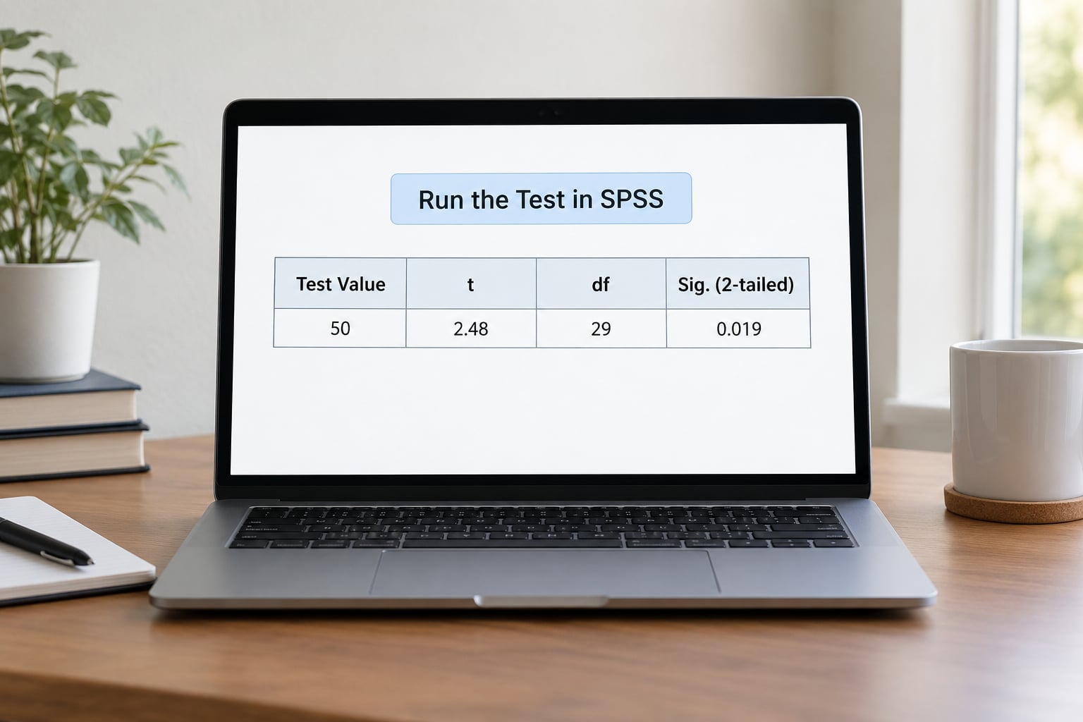
Click Analyze > Compare Means and Proportions > One-Sample T Test. Move your outcome into the Test Variable(s) box and type the benchmark into the Test Value box. The default confidence interval is 95%, which is what you want unless your course says otherwise.

Tick Estimate effect size under Options if you want Cohen’s d and Hedges’ g. In older versions this is the only effect size on offer; version 27 and later give you a row of standardised measures. Then click OK.

For readers without SPSS, the same test is one line in R: ttest(x, mu = 5, alternative = "two.sided"). In Excel, Data > Data Analysis > t-Test: One-Sample for Two-Tailed for Tests, type the test value in the box labelled that way, and check Summary. JASP and jamovi put it under T-Tests > One Sample T-Test.

5. Interpret the Output

SPSS prints two tables. The One-Sample Statistics table gives you N, Mean, Std. Deviation and Std. Error Mean. The One-Sample Test table gives you the row you actually report: Test Value, t, df, Sig. (2-tailed), Mean Difference, and the 95% Confidence Interval of the Difference as Lower and Upper.

Here is a complete worked example you can reproduce. Thirty students rate a training programme on a 1 to 10 scale, and you want to know whether their average differs from a neutral benchmark of 5.

• N = 30, Mean = 6.42, Std. Deviation = 1.38, Std. Error Mean = 0.25
• Test Value = 5.00, Mean Difference = 1.42
• t(29) = 5.64, Sig. (2-tailed) = .000
• 95% CI of the Difference: [0.91, 1.93]
• Cohen’s d = 1.03

Check it by hand and you get the same number: t = (6.42 – 5.00) divided by (1.38 divided by the square root of 30), which is 1.42 / 0.252 = 5.64. If your software disagrees with your arithmetic, something is wrong with the data setup, not the statistics.

Now interpret. Compare Sig. (2-tailed) with your alpha of .05. Here .000 is below .05, so you reject the null. The direction comes from the sign of t and the Mean Difference: positive means the sample mean sits above the test value.

Sig. (2-tailed) = .000 does not mean p equals zero. SPSS prints three decimals, so .000 actually means p is less than .0005. Never copy .000 into a write-up; report p < .001.

Read the confidence interval too. Here the whole interval sits above zero, which confirms the sample mean is reliably above 5.00. An interval that straddles zero means the difference is not distinguishable from no difference, whatever the p value says.

One more caution. A significant result says the difference is unlikely to be chance noise, not that it matters. A 0.3-point difference on a ten-point scale can be highly significant in a large sample and irrelevant in practice. Always report the mean difference or the interval so a reader can judge.

6. Report the Result in APA Style

APA 7 wants a single sentence in the body text, in this order: test name, the abbreviations, test value, t, degrees of freedom in parentheses, p, the effect size, and the confidence interval. Mean and standard deviation go in the sentence too if your assignment asks for descriptives.

A one-sample t-test showed that training ratings (M = 6.42, SD = 1.38) were significantly greater than the benchmark of 5.00, t(29) = 5.64, p < .001, 95% CI [0.91, 1.93], d = 1.03.

For a non-significant result, say so plainly and give the interval rather than pretending the effect vanished. Here is the matching example: eighteen participants score 4.88 on average against the same benchmark, giving t(17) = -0.55, p = .586, 95% CI [-0.58, 0.34], d = -0.13.

A one-sample t-test indicated that quiz scores (M = 4.88, SD = 0.92) did not differ significantly from the pass mark of 5.00, t(17) = -0.55, p = .586, 95% CI [-0.58, 0.34].

Seven formatting rules cover almost every marker I have seen deduct points for. Round means, standard deviations and t to two decimals, and always keep the leading zero on t (t = 5.64, never t = .64). Report p to two or three decimals with no leading zero (p = .003, never p = 0.003), and convert .000 to p < .001. Give degrees of freedom as an integer, keep the italic t but not the italic p, and italicise the statistical symbols t, M, SD, p, n and CI. Always say two-tailed or one-tailed explicitly rather than leaving the reader to guess.

If you want a table as well, APA 7 allows a copy-ready one:

Statistic	M	SD	t	df	p	d
Training rating vs 5.00	6.42	1.38	5.64	29	< .001	1.03

Do not paste the raw SPSS screenshot into your document. Rebuild the numbers in a clean table and keep the output file for your appendix.

Common Mistakes

Using an independent-samples t-test is the most common wrong turn. That test compares two groups to each other; you have one group and a benchmark. If you find yourself in the Independent-Samples dialog, you are on the wrong path.

Choosing the test value after seeing your data is a design error, not a formatting one. It inflates significance and a marker will spot it, especially when the “benchmark” turns out to be suspiciously close to your mean.

Switching to one-tailed after the two-tailed p value comes back at .08 is the same mistake wearing a hat. Choose your alternative before running, and justify it with theory. SPSS always gives you the two-tailed value, so halving it by hand is a red flag in a submitted document.

Ignoring assumptions is common because the test still produces output. Report the checks you ran. One line is enough: “Normality was confirmed with a Shapiro-Wilk test, W(29) = .96, p = .19, and no outliers were present.”

Omitting the effect size is increasingly penalised in APA 7 courses. Cohen’s d is cheap to obtain and tells the reader how big the difference was in standard deviation units.

Reading a non-significant result as proof of no difference is the most common interpretive error. It only means the data were too thin to detect one. The confidence interval shows the range of differences still consistent with your data, and that range is often wide enough to matter.

Finally, running many one-sample t-tests on the same sample inflates your chance of a false positive. Five tests at .05 give roughly a 23% chance of at least one spurious hit. If you run several, correct with a Bonferroni adjustment or say so in a limitations paragraph.

Practical Tips and Reporting Checklist

Run through this before you submit. It catches most of what markers dislike.

• Your variable is continuous and its measurement scale is set to Scale.
• The test value has a citation: an author, a year, or a published standard.
• The null and alternative hypotheses are stated in your methods section, before any results.
• You ran a boxplot and a normality check, and you report both, including the failed ones.
• You report N from the statistics table, not the number of rows you typed.
• t has two decimals and a leading zero; p has no leading zero and is never .000.
• The effect size and the 95% confidence interval appear in the results sentence.
• You say two-tailed explicitly.
• Your sentence states the direction, not just significance.
• You kept the output file, because a supervisor may ask where the numbers came from.

Two habits save time later. Save your output as a separate file with a sensible name the moment you run anything, and write the results sentence while the table is still on screen. Reconstructing t and df from a printout twenty pages later is nobody’s idea of a good evening.

Finally, tie the result back to your research question in one closing sentence. A test that answers a question nobody asked is a number in a vacuum, and readers cannot tell whether the finding matters without that link.

Frequently Asked Questions

Conclusion

Start by confirming you have one continuous variable and a benchmark you can cite. Check the boxplot and normality test, run Analyze > Compare Means and Proportions > One-Sample T Test, then write the result with t, df, p, the confidence interval and an effect size, formatted to two decimals with no leading zero on p. That sequence takes ten minutes and covers almost everything a marker looks for.