
To run a Fisher exact test in SPSS, open Analyze, Descriptive Statistics, Crosstabs, put your two categorical variables in the Row and Column boxes, then tick Fisher’s exact test under Statistics. Reach for it when any expected cell count in your contingency table falls below 5, because that is where the chi-square approximation breaks down.
It takes about ten minutes end to end, most of which is checking that your variable coding has not silently merged two categories. I have watched an entire analysis get thrown out because “Non-smoker” and “Never smoked” had been collapsed into one value during data entry.
Below is the SPSS route in full, then a worked example you can recompute by hand, and then the interpretation and reporting steps that usually cause the trouble.
Table of Contents
- 1What You Need
- 2When to Use Fisher’s Exact Test
- 3The three-condition rule for choosing Fisher over chi-square
- 4What the three tests do with the same table
- 5How to Run a Fisher Exact Test in SPSS
- 6Step 1: check the coding before anything else
- 7Step 2: open the Crosstabs dialog
- 8Step 3: switch on the exact test
- 9Step 4: ask for the expected counts
- 10Step 5: add the effect size
- 11Step 6: check the output
- 12Worked Example: One Table From Counts to Conclusion
- 13How to Interpret the SPSS Output
- 14Reading the odds ratio
- 15How to Report Fisher’s Exact Test Results
- 16Common Mistakes
- 17Frequently Asked Questions
- 18When should I use Fisher’s exact test?
- 19When should I not use Fisher’s exact test?
- 20Does Fisher’s exact test give an odds ratio?
- 21How do I interpret an odds ratio of 1, 3 and 0.5?
- 22How do I report Fisher’s exact test results in APA?
- 23How do I run the same test in R, Stata or Python?
- 24Conclusion
What You Need

You need two things that are categorical, and a dataset where every case is independent of every other case. That rules out continuous variables, ordinal scores treated as continuous, and anything measured on a scale where the gaps between values are meaningful.
Both variables need at least two categories, and the cells of the resulting contingency table hold counts of people, not means or percentages. Twenty people answering yes or no on two questions gives you a 2×2 table with four counts in it.
Independence matters more than people expect. If the same participant answered both questions, or if each person contributed several observations, the test is answering the wrong question. For paired binary data, McNemar’s test is the right tool instead.
You also need to know where the decision threshold sits. The rule of thumb is that the chi-square test is fine when all expected counts reach 5 or more, and Fisher’s exact test takes over when any expected count drops below that. Expected counts are what you would expect to see if there were no association at all, not the counts you actually have.
On the software side, the exact test lives in the base module of IBM SPSS Statistics, so no add-on licence is required. If your Statistics dialog has no Exact button to press, check the release you are running before the rest of this applies.
When to Use Fisher’s Exact Test
Fisher’s exact test is a test of independence for two categorical variables. It works by holding the row and column totals fixed and working out the probability of every arrangement of the data that could have produced those totals, using the hypergeometric distribution. The p-value is the sum of the probabilities of all arrangements at least as extreme as the one you observed. Nothing is approximated.
The three-condition rule for choosing Fisher over chi-square
- Both variables are categorical, with two or more categories each.
- Observations are independent, so no participant contributes twice.
- One or more expected cell counts fall below 5, which usually happens with small samples or rare events.
That third condition is the one that gets misread. It is about expected counts, not observed counts and not total sample size. A platform experiment with 200,000 visitors and 11 purchases in one arm has tiny expected counts even though nothing about the sample is small.
What the three tests do with the same table
Pearson chi-square relies on a large-sample normal approximation, and with sparse cells its p-values come out too small, which inflates false positives.
Chi-square with Yates continuity correction uses the same approximation with a correction applied, and on sparse tables it over-corrects, pushing p-values too high.
Fisher’s exact test assumes nothing beyond independent counts. It stays valid at any table size, but it is conservative.
Conservative means the real type I error rate sits below the nominal 5 percent, so the test is reluctant to declare significance. That is the price of validity. You will occasionally get a p-value above .05 where a chi-square test would have squeaked under, and that result is still the honest one.
For a 2×2 table the degrees of freedom are always 1, so the chi-square approximation problem applies to every Fisher-eligible table you will ever build. Smallness of expected counts, not the degrees of freedom, is the actual trigger.
How to Run a Fisher Exact Test in SPSS
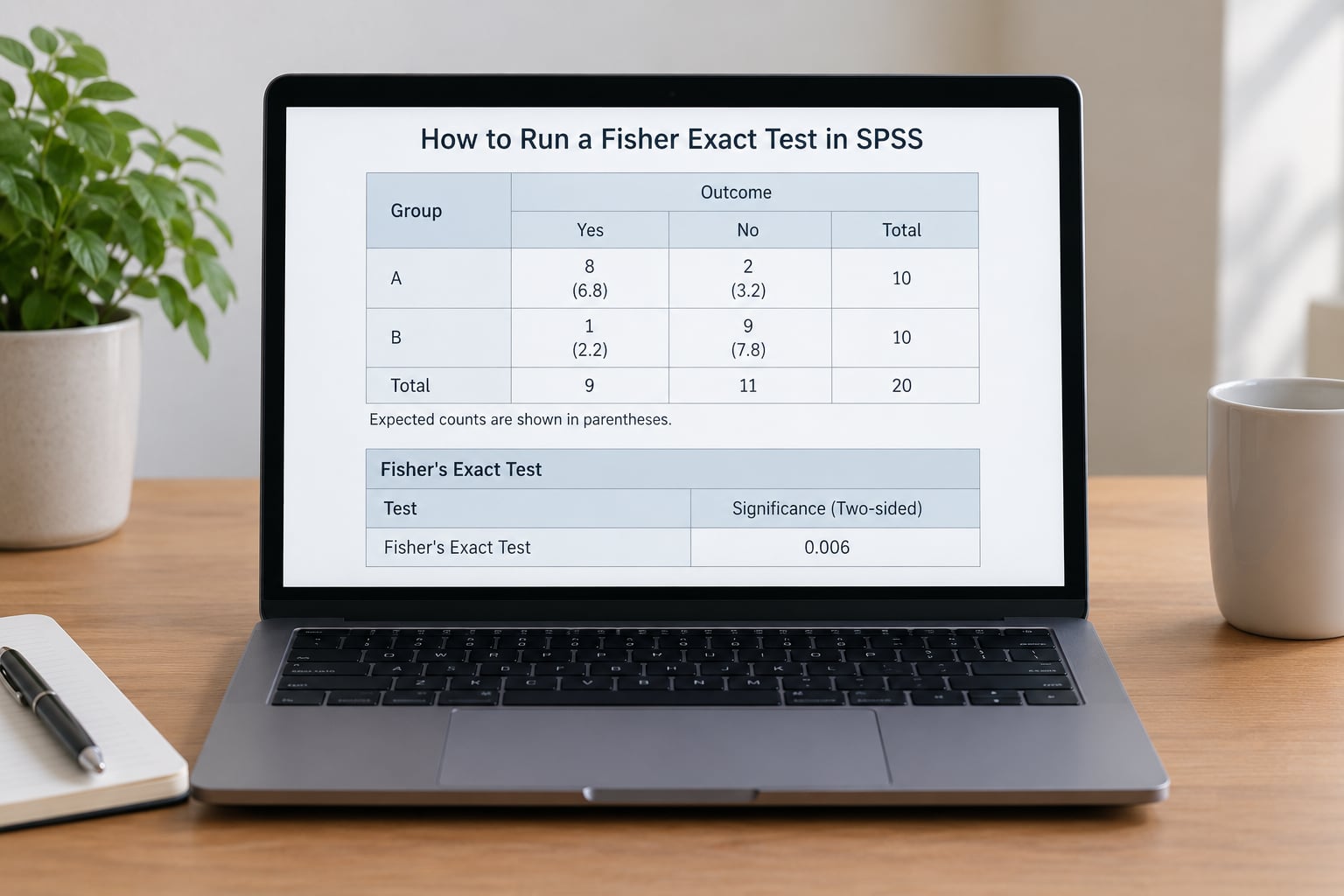
Step 1: check the coding before anything else
Open Frequencies for each variable and look at the Values and Labels list. What you want is a small, clean set of categories with counts that add up to your sample size. If a category is missing, decide now whether those cases belong in an Other group or out of the analysis entirely, and record that decision.
Step 2: open the Crosstabs dialog
Go to Analyze, then Descriptive Statistics, then Crosstabs. Put the outcome variable in the Row box and the predictor in the Column box. Either orientation gives the same p-value, but the odds ratio direction flips, so pick the arrangement that makes your table read the way you want to describe it.
Step 3: switch on the exact test
Click Statistics in the dialog. Tick Fisher’s exact test. If your table is exactly 2×2, SPSS also offers an Exact button that opens a small panel reporting the two-sided and one-sided significance values separately, which is more useful than the single figure in the main test box. Click Continue.
Step 4: ask for the expected counts
Click Cells, tick Observed and Expected, then Continue. Without this you cannot see whether the expected-count rule applies, and you are choosing the test on faith.
Step 5: add the effect size
If your table is 2×2, tick Relative Risk in the same Statistics panel. That adds a Risk table with an odds ratio and its confidence interval. The odds ratio is an estimate computed separately from the exact test, which is fine, but you should know it is a large-sample style estimate and can be badly behaved when a cell holds a zero or a one.
Step 6: check the output
The Output Viewer gives you three things to look at. The crosstabulation with expected counts underneath tells you whether Fisher was the right call. The Fisher’s Exact Test box gives the two-sided significance, which is the number you report. The significance of your chosen test, at the top, is the one that matches your plan.
If your data is already in aggregated form, that is, a table of counts rather than one row per person, load the counts into Data View first and use Data, Weight Cases, Weight by frequency. Running raw counts as if they were cases is a common and very quiet error.
Readers working in other packages can reach the same result. In R, build the table with matrix() and call fisher.test(). In Stata, tabi works directly on the four cell counts. In Python, scipy.stats.fisher_exact takes the same 2×2 array. All four give the identical p-value for the same table.
Worked Example: One Table From Counts to Conclusion
Suppose a pilot trial has 12 patients on the treatment and 8 on placebo. Nine of the 12 treated patients improve, and 2 of the 8 placebo patients do. That gives you four observed counts: 9, 3, 2 and 6.
                    Improved   Not improved   Total
Treatment                 9              3       12
Placebo                   2              6        8
Total                    11              9       20
Now compute the expected counts by multiplying each row total by each column total and dividing by 20. The treated-and-improved cell expects 12 x 11 / 20 = 6.6, and treated-not-improved expects 5.4. Down in the placebo row the two expected counts are 4.4 and 3.6.
Two of those four expected counts fall below 5, so the chi-square approximation is not safe here and Fisher’s exact test is the correct choice. That calculation is the entire decision, and you can do it in your head before ever opening SPSS.
Running the table in SPSS gives a two-sided exact p-value of .041 and a one-sided value of .040. For comparison, the uncorrected Pearson chi-square on the same counts is 4.85 with a p-value of .028, while the Yates-corrected version is 3.04 with a p-value of .081.
Two of those three tests fall below .05 and one does not, which is precisely the situation that tempts people into reporting whichever they prefer. Report the one the expected counts selected. Here that is Fisher’s exact, p = .041.
The odds ratio works out to (9 x 6) divided by (3 x 2), which is 9.00, with a 95 percent confidence interval running from about 1.14 to 71.00. The point estimate says the odds of improvement are nine times higher on treatment, and the interval barely clears 1, which tells you plainly how little 20 cases can pin down.
How to Interpret the SPSS Output
Start with the two-sided significance. It is the default in SPSS, it is what almost every journal expects, and it is the value you report unless you committed to a directional hypothesis in advance. A two-sided p of .041 means that, if the two variables were genuinely unrelated, tables at least this far from chance would come up about 4 times in 100 pure repetitions of this design.
The one-sided value is usually close to the two-sided one when the observed counts sit right at the edge of what the margins allow, which is exactly what happened in the example above. Halving a two-sided p-value after seeing that your result is significant is a one-sided test chosen with knowledge of the outcome, and it inflates your error rate. Decide the direction in your proposal, not at the output window.
Reading the odds ratio
An odds ratio of 3 means the odds of the outcome are three times higher in one group than the other. It is not three times higher risk. Odds and risk diverge sharply once the event is common, so if your outcome affects more than about 10 percent of people, report the relative risk instead and keep the odds ratio for the sparse tables it suits.
An odds ratio of 1 means no difference. Above 1 points to the group in the numerator, below 1 to the other. Values further from 1 mean a stronger association, and the confidence interval tells you how precisely you know it. A wide interval spanning 1 means the direction is plausible but the size is not pinned down, which is the normal state of affairs in a small sample.
What the test cannot tell you is why the two variables are associated. It rules out or fails to rule out independence given the margins, and nothing more.
How to Report Fisher’s Exact Test Results
Report the test, the p-value, and the effect size with its interval. The APA notation for an exact p-value is p = .041, and you do not attach a degrees of freedom value, because there is no chi-square statistic to attach it to.
A filled sentence reads like this: a Fisher’s exact test showed that patients receiving treatment improved significantly more often than those on placebo, 9 of 12 compared with 2 of 8, p = .041, odds ratio = 9.00, 95 percent confidence interval [1.14, 71.00].
In a results table, give the raw counts rather than percentages, because percentages hide the small denominators that justified the exact test in the first place. Label the columns with the group names so the sentence and the table agree on direction.
Keep the interpretation descriptive. Treatment groups are not assigned by a randomizer in a case-control study, so the odds ratio describes an association and does not license a causal claim. Where randomisation is genuinely present, you can go further, and you should say so plainly.
Common Mistakes
The first mistake is applying the expected-count rule to observed counts. A cell showing 6 looks reassuring while the expected count underneath it sits at 3.6, and the test is invalid. Always read the expected row in the output.
The second is treating exact as more accurate. It is exact with respect to the enumeration, and conservative in its decisions. Reporting a Fisher p-value as a more precise estimate of the truth is a claim the method does not support.
The third is running chi-square and Fisher on the same table and reporting whichever one falls below .05. Because the two tests disagree most often right around the threshold, that practice buys significance at a real cost in false positives. Choose the test from the expected counts, write it down, and report it whatever it says.
The fourth is reaching for the one-sided option because the two-sided result sat near the line. That choice made after seeing the data is not a hypothesis test anymore.
The fifth is ignoring independence. Repeated measures, before and after designs, and matched pairs all break the assumption quietly, and McNemar’s test is the usual replacement for paired binary data.
The sixth is overlapping category labels in SPSS. If two value labels map to the same value, cases drop out of the table without a warning, and the resulting p-value describes a smaller sample than the one in your methods section. Check the N row in the output against your expected N every time.
Finally, remember that exact p-values above 0.5 are not reported by every package, and R and SPSS can differ slightly because they define “more extreme” differently. If you are cross-checking two programs and land on a small discrepancy in the third decimal, that is usually the reason, not an error.
Frequently Asked Questions
When should I use Fisher’s exact test?
Use it when you have two categorical variables with independent observations, and at least one expected cell count in the contingency table falls below 5. Expected counts are what you would expect under no association, not the counts you actually recorded. Small samples and rare events both produce this pattern, and either one is enough reason to switch away from the chi-square test.
When should I not use Fisher’s exact test?
Skip it when your data are continuous rather than categorical, when the same participants appear more than once, or when the outcome and predictor are the same variable measured twice. Do not use it merely because you want a smaller p-value. Some software also has a computation limit for tables larger than 2×2, where a Monte Carlo approximation of the same exact test is the practical route.
Does Fisher’s exact test give an odds ratio?
The test itself produces only a p-value, but an odds ratio usually accompanies it. In SPSS, tick Relative Risk in the Crosstabs Statistics panel to add a Risk table containing the odds ratio and its confidence interval. In R, fisher.test() returns the odds ratio by default, along with a conditional maximum likelihood interval that is usually narrower and better behaved than the Wald interval.
How do I interpret an odds ratio of 1, 3 and 0.5?
An odds ratio of 1 means the two groups are equally likely to show the outcome. A value of 3 means the odds are three times higher in the group in the numerator of the ratio. A value of 0.5 means the odds are halved in that same group. None of these are risk ratios, and the two diverge noticeably once the outcome is common, so report relative risk for frequent outcomes.
How do I report Fisher’s exact test results in APA?
Name the test, give the exact p-value, and add the effect size with its interval. Write p = .041 with no equals-attached statistic and no degrees of freedom, because no chi-square value was computed. A typical sentence names the groups, quotes the raw counts, and closes with the p-value and odds ratio. Do not describe the association as causal unless the design supports it.
How do I run the same test in R, Stata or Python?
In R, build the table with matrix(c(9, 3, 2, 6), nrow = 2, byrow = TRUE) and pass it to fisher.test(). In Stata, type tabi 9 3 2 6, which expects the four cell counts in that order. In Python, call scipy.stats.fisher_exact on the same 2×2 array. All three return the same two-sided p-value for the same table.
Conclusion
Check the design before the software. Two categorical variables, independent cases, and at least one expected count under 5 is the whole decision, and it takes a pencil and the Cells dialog to confirm.
Then run it from Analyze, Descriptive Statistics, Crosstabs, tick Fisher’s exact test under Statistics, read the two-sided significance, and cross-check it against the expected counts row you printed in Step 4. Report that number as p = .041 with no degrees of freedom, add the odds ratio with its interval, and describe the association without claiming a cause. That is the complete answer to how to run a Fisher exact test and when to use it, and it takes ten minutes to do properly.