How to Use Open Street Map Data in a Research Project (2026)

To use OpenStreetMap data in a research project, you frame a geographic question, pull only the tagged features you need from a bounded study area, validate them against an authoritative source, and turn them into variables your statistics can test. The whole thing takes a day to set up for a single-city study, but the quality checks are what separate a publishable result from a map that only looks convincing.

OpenStreetMap is a volunteer-built geographic database, so it is free, global and far more detailed than most commercial layers available to a student. That same volunteer origin is also its weakness: coverage is uneven, tags change weekly, and completeness varies enormously between a dense city centre and a rural district. This guide walks the full path from research design to reported findings.

Table of Contents

1. 1What You Need
2. 2Step-by-Step
3. 31. Define a research question and study boundary
4. 42. Identify the OpenStreetMap features you need
5. 53. Download or extract the data
6. 64. Inspect and document data quality
7. 75. Clean and standardise the spatial data
8. 86. Create measurable variables for analysis
9. 97. Analyse the data with statistical or spatial methods
10. 108. Produce clear maps and supporting tables
11. 119. Interpret, validate and report the findings
12. 12Common Mistakes
13. 13Treating tags as verified attributes
14. 14Querying an unbounded area
15. 15Ignoring local mapping activity
16. 16Using the wrong spatial unit
17. 17Treating road distance as travel distance
18. 18Not recording the extraction date
19. 19Overstating precision
20. 20Omitting attribution and uncertainty
21. 21Frequently Asked Questions
22. 22How can I download OpenStreetMap data?
23. 23How accurate is OpenStreetMap data?
24. 24How do I check OpenStreetMap data completeness before using it?
25. 25How do I cite OpenStreetMap in my research?
26. 26Why is my Overpass query timing out?
27. 27Is OpenStreetMap data biased?
28. 28Conclusion

What You Need

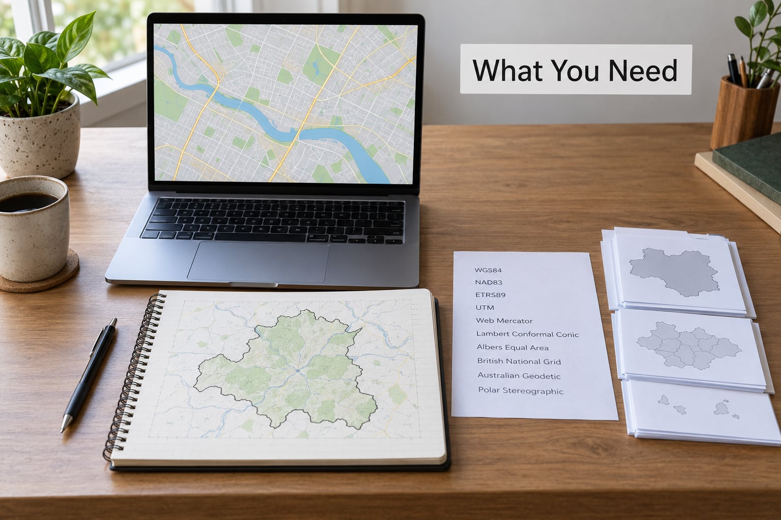
Before any download, six things need to be written down, and every later decision depends on them.

1. The research question. Something you can measure with geometry. “Is the city walkable?” is too broad; “Are primary-school catchments associated with street connectivity” is answerable.
2. The study area, as a bounding box of minimum and maximum longitude and latitude, or an administrative polygon you have already obtained. Decide this now, not after you realise your extract covers three countries.
3. The feature types you need — roads, buildings, waterways, land use, public transport stops, healthcare facilities, schools, accessibility barriers such as steps and kerbs.
4. The unit of analysis. A point, a line, a polygon, or an aggregate zone such as a neighbourhood, grid cell or administrative ward. This choice constrains every variable you can build later.
5. Spatial software. QGIS for visual inspection, plus either R or Python for scripted extraction and analysis.
6. A documentation file. Start it now. It becomes your methods section.

Keep OpenStreetMap-created geodata separate from other GIS layers you plan to use — census boundaries, satellite imagery, national registers. Provenance and licence terms differ, and mixing them in a single layer without tracking origin creates attribution problems later.

Check the licence before you build anything. OpenStreetMap data is released under the Open Database License, which requires attribution and imposes share-alike conditions on derived databases. Commercial and institutional users should read the licence text rather than relying on a blog summary.

Step-by-Step

1. Define a research question and study boundary

Turn a broad interest into a question with a measurable outcome, a defined population and a geographic frame. Record the population, the period covered, and the spatial extent.

Choose the unit of analysis first, because it decides what counts as evidence. Points suit facilities and incidents. Lines suit networks and accessibility. Polygons suit land use, buildings and administrative areas.

Using a bounding box rather than an administrative boundary is usually the cleaner start. A rectangle is unambiguous, easy to reproduce and does not depend on administrative data you have not verified yet. You can clip to real boundaries in a later step.

How to tell it worked: someone else reading your methods section could draw the same study area from your coordinates without asking you a question.

2. Identify the OpenStreetMap features you need

Map each part of your question to a tag. Research on healthcare access needs amenity values for doctors, clinics and hospitals. Walkability work needs highway classes plus footway detail. School catchments need amenity=school, and school accessibility often needs barrier values such as kerb and steps.

Inspect tags before committing to them. Open a few candidate objects in the OSM data browser and read the full key-value set. Real objects carry secondary tags that a naive filter discards, and discarding them can quietly change your count.

Watch for near-synonyms. The same clinic may be tagged amenity=doctors, amenity=clinic or healthcare=centre. A query that handles only one of those under-counts, and it under-counts unevenly across regions where different tagging conventions dominate. This is the single most common reason an OSM amenity count disagrees with a council’s official list.

3. Download or extract the data

There are three practical routes, and the right one depends mostly on how large your study area is.

Route	What you get	Best for	Watch out for
Overpass API query	Only the elements matching your tags, as JSON or XML	Single city, district or study zone; anything up to roughly an urban area	Shared public servers are rate-limited; widen the box too far and the query times out
Regional extract (Geofabrik-style PBF)	The complete current state of a region as a compressed file	Several cities, a whole country, or analyses needing tag combinations you did not anticipate	Large files need filtering before they will fit in memory; update lag of a day or more
Full planet file	Everything, worldwide	Multi-country comparative work with proper hardware	Enormous download and substantial memory; almost never the right first move for a thesis

Whichever route you take, save the exact query text beside the output. A query you cannot re-run is not a method, it is an anecdote.

Two practical notes. First, if your area is a place name rather than coordinates, geocoding it can return several candidates with the same name in different countries; inspect the candidate list and confirm you have the right one before you use its bounding box, because a wrong box silently corrupts an entire study. Second, always request one element group at a time rather than accepting everything a query returns, otherwise relation members and ferry routes tagged as highways drift into your results and inflate your counts.

How to tell it worked: your feature count is plausible against a rough mental model of the area, and a zoomed-in map of the output shows features inside the rectangle and nothing wildly outside it.

4. Inspect and document data quality

Three quality dimensions are distinct, and conflating them is the most common methodological error in OSM research.

Dimension	The question it answers	A practical check
Completeness	Are the features that exist actually present?	Compare counts against an authoritative source — a national building register, a council asset list — and report the overlap percentage and how you computed it
Positional accuracy	Are the coordinates right?	Overlay a sample of geometries on aerial imagery or cadastral data and measure offset on a subset
Temporal recency	Does it reflect the period you claim?	Check timestamp and version fields; inspect how recently the area was edited, since local mapping activity varies enormously

Report the completeness figure you actually computed. A stated percentage with a method behind it is worth far more than a confident claim that the data is accurate. Researchers who compare OSM building footprints against an authoritative flood-modelling source have shown the value of exactly this check — and the value of reporting where the data falls short.

Then consider bias. Volunteer mapping concentrates where volunteers live, travel and work, so coverage skews toward wealthy urban and tourist areas and thins out in places that matter socially. Treat a low-density area as possibly unmapped rather than genuinely empty. Academic users consistently treat OSM as a complement to authoritative data, never as a substitute without validation.

How to tell it worked: your documentation file now contains a completeness estimate, a note on positional accuracy, and a stated list of limitations.

5. Clean and standardise the spatial data

Convert to a simple-features format your software reads natively. Repair invalid geometries, drop duplicate geometries that arise from repeated ways, and standardise tag values so that synonymous spellings collapse into one category.

Handle missing tags explicitly rather than letting them default to zero in a later count. A feature with no opening_hours is not a facility that never opens. Deciding between excluding those records, treating them as a separate category, and reporting the proportion missing is a research decision, not a formatting one.

Clip to your study boundary and settle on a coordinate reference system before any distance or density calculation. A bounding box in longitude and latitude is fine for storage and web maps; measuring metres in degrees produces nonsense at high latitudes, so project to a metric or appropriate local system first.

Archive an extract alongside the results. Snapshot the files, note package versions, and keep a timestamped copy so you can regenerate the same dataset later.

Reproducibility checklist — archive all of this with every extract:

• The exact query text, saved as a file
• The bounding box coordinates or boundary relation id
• The retrieval timestamp, to the minute
• The list of osm_id values returned
• Software and package versions
• The attribution and licence string you will print with the output

How to tell it worked: a colleague can re-run your extract on a different machine and get the same feature set. If the database has moved on since, your archived ids and files still let them reconstruct what you analysed.

6. Create measurable variables for analysis

Raw geometry is not a variable. Convert features into something your statistics can take: counts per zone, distance to the nearest facility, network travel time along actual routes rather than straight lines, densities per square kilometre, intersections per kilometre of road, or coverage within a stated walking radius.

Pick the aggregation that matches your unit of analysis — neighbourhood, grid cell, administrative area or sampling point. A regular grid avoids the problem of zones with wildly different sizes, which otherwise makes raw counts misleading.

Watch the difference between crow-flight and network distance. Two kilometres in a straight line can be three on foot if a river or a motorway sits between. Network-based distance requires routing software; straight-line distance is an approximation and should be labelled as one.

How to tell it worked: every variable has a stated unit, a stated denominator where relevant, and a plausible range.

7. Analyse the data with statistical or spatial methods

Join your OSM-derived variables to survey responses, census counts or observations, then analyse in R, Stata, SPSS, Python or QGIS. Start with descriptive comparisons — means, distributions, maps — before reaching for anything heavier.

From there, correlations and regression handle the relationship between a mapped variable and an outcome. Clustering is useful for grouping zones by their mapped characteristics. Network analysis suits accessibility questions. Spatial statistics matter more than most tutorials admit: if neighbouring areas share a mapped attribute, your observations are not independent, and ordinary regression will report narrower standard errors than the data supports. Moran’s I on your residuals is a quick check on that.

Two interpretation warnings. Ecological fallacy is the big one — a correlation between a zone-level amenity count and a zone-level outcome says nothing about the individuals inside that zone. Boundary-related effects are the second: results shift depending on where you draw the study edge, so test sensitivity to that choice.

How to tell it worked: you can state, for every claim, which variables entered the model and at what level of aggregation.

8. Produce clear maps and supporting tables

Choose a map type that matches the message: a choropleth for a rate or a normalised value, a proportional-symbol map for counts, a network map for connectivity, a point layer for facility locations.

Classify values honestly. Natural-breaks classifications exaggerate differences between similar zones; quantiles force every class to hold the same number of observations. Whatever you choose, say which method you used in the caption. Every map needs a title, a legend, a scale where relevant, a source line naming OpenStreetMap with the retrieval date, and a note on data quality.

A map that dumps raw points onto a basemap is not a result, it is a screenshot. If the reader cannot extract the finding from the figure alone, the analysis has not finished.

9. Interpret, validate and report the findings

Check your results against independent sources — official statistics, local knowledge, aerial imagery — and be explicit when they disagree. Then ask whether your conclusion survives a reasonable alternative specification: a different buffer distance, a different aggregation, a different completeness threshold.

Distinguish association from causation throughout. Mapped variables correlate with all kinds of unmeasured things, and volunteered data carries its own selection patterns into the relationship.

Document the full pipeline: the query, the filters, the transformations, the software versions, the analysis steps. Report the limitations as findings in their own right — the completeness estimate, the coverage bias, the boundary sensitivity. Other researchers then know exactly how far to trust the result.

How to tell it worked: someone can read your paper, re-run your extract and your analysis, and get the same numbers.

Common Mistakes

Treating tags as verified attributes

A tag records what a contributor believed at a moment in time. It is a claim, not a measurement. Validate sampled features against imagery or an official register before treating a tag as ground truth.

Querying an unbounded area

Running a query over a whole region, or no region at all, is why people hit timeouts and memory errors. Always bound the query. If the box must grow, split it into tiles, extract each, and merge.

Ignoring local mapping activity

Coverage is not uniform, and a district with few mapped features may simply have few contributors rather than few buildings. Check the density of recent edits in the area and report it.

Using the wrong spatial unit

Analysing amenity counts without normalising by area or population produces a map of where people live, not of service provision. State the denominator.

Treating road distance as travel distance

Straight-line buffers over rivers, walls and motorways are wrong in ways that bias the results systematically in certain neighbourhoods. Route along the network, and say which method you used.

Not recording the extraction date

The database changes every minute. Without a timestamp, your result cannot be regenerated or defended, and this is the most frequently cited criticism of published OSM research.

Overstating precision

Reporting amenity counts to six decimal places implies accuracy the source cannot support. Round to what your completeness estimate justifies, and report that estimate.

Omitting attribution and uncertainty

The Open Database License requires attribution, and a derived database carries share-alike obligations. Put the required credit on every figure and in the references, and state the data-quality caveats next to the results rather than in a footnote nobody reads.

Frequently Asked Questions

Conclusion

Start here: write the geographic question and its unit of analysis in one sentence, set a bounding box, pick the specific tag values you will query, then save the query text and the retrieval timestamp with your first extract.

After that, measure completeness against an authoritative source, sample positional accuracy, and document what you find. The rest of the workflow — variables, statistics, maps — is straightforward once those three pieces are done, and skipping them is what makes an OpenStreetMap result hard to defend.