How to Calculate NDVI from Satellite Imagery (October 2026)

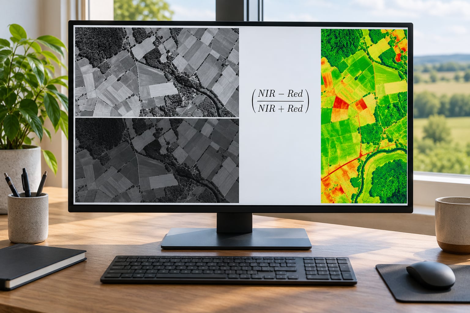
To calculate NDVI from satellite imagery you subtract red reflectance from near-infrared reflectance and divide that difference by the sum of the two: NDVI = (NIR – Red) / (NIR + Red). You need two bands from the same image, on the same pixel grid, in reflectance units. The whole process takes about 20 minutes once the imagery is downloaded, and the only genuinely hard part is catching the few errors that produce a plausible-looking but wrong map.

Here is the whole workflow in seven steps:

1. Choose a cloud-free image from a sensor that gives you a red band and a near-infrared band.
2. Open the band metadata and confirm the band numbers, wavelengths, scaling factor and pixel size.
3. Load the red and NIR bands and confirm they actually cover your study area.
4. Resample or align both bands to one grid and apply a valid-data or cloud mask.
5. Apply (NIR – Red) / (NIR + Red) with a guard on the denominator.
6. Check the output: values should fall between -1 and +1, and vegetation should read positive.
7. Export the NDVI raster as a GeoTIFF and write down the sensor, date and bands you used.

The rest of this guide fills in each of those steps, including the software menu paths for QGIS and ArcGIS Pro, a Google Earth Engine version that runs entirely in the cloud, and a short Python route for when you need to repeat the calculation across many dates.

Table of Contents

1. 1What You Need
2. 2Step-by-Step
3. 3Step 1: Choose Suitable Satellite Imagery
4. 4Step 2: Inspect the Band Metadata
5. 5Step 3: Load and Inspect the Red and NIR Bands
6. 6Step 4: Align the Bands and Mask Invalid Pixels
7. 7Step 5: Apply the NDVI Formula
8. 8Step 6: Check the NDVI Results
9. 9Step 7: Export and Document the NDVI Raster
10. 10Common Mistakes
11. 11Reversed bands in the formula
12. 12Integer division truncating the result
13. 13Mismatched pixel grids
14. 14Cloud and shadow contamination
15. 15Unmasked no-data values
16. 16Values outside the -1 to +1 range
17. 17Tips for Reliable NDVI Results
18. 18Frequently Asked Questions
19. 19Can I calculate NDVI from a normal satellite image?
20. 20Which bands should I use for Landsat and Sentinel-2 NDVI?
21. 21Do NDVI values always range from -1 to 1?
22. 22Should I cloud-mask satellite imagery before calculating NDVI?
23. 23Why are my NDVI results all zero, blank, or outside the expected range?
24. 24Which GIS software is easiest for calculating NDVI?
25. 25Conclusion

What You Need

NDVI is a measure of how green vegetation is, derived from how strongly a surface reflects two parts of the spectrum. Healthy plant canopy absorbs red light for photosynthesis but reflects most of the near-infrared light hitting it, so the two bands pull apart and the ratio goes positive.

Before you open any software, gather five things:

• An image with a red band and a near-infrared band. Every mainstream optical satellite has both, but they are numbered differently per sensor.
• The band metadata from the imagery documentation: band numbers, wavelength ranges, the reflectance scaling factor, spatial resolution and the no-data value.
• A GIS tool. QGIS and ArcGIS Pro both have a raster calculator. Google Earth Engine does the whole thing in the browser. Python with rasterio and numpy does it in a script.
• Both bands on the same pixel grid. The red and NIR rasters must share a coordinate reference system, extent, cell size and origin, or your pixels will be compared against the wrong locations.
• A valid-data or cloud mask. Pixels that are no-data, saturated, clouded or in shadow produce meaningless NDVI unless you remove them first.

One more thing worth deciding early: whether you want top-of-atmosphere reflectance from a Level-1 product or bottom-of-atmosphere surface reflectance from a Level-2 product. For most crop and vegetation work, Level-2 surface reflectance is the better choice because the atmosphere has already been corrected.

Step-by-Step

How to calculate NDVI from satellite imagery comes down to four operations repeated carefully: pick the right bands, put them on one grid, do the arithmetic in floating point, and verify the result before you trust it. Work through the steps below in order rather than jumping straight to the calculator, because most broken NDVI maps are broken upstream of the formula.

Step 1: Choose Suitable Satellite Imagery

Pick a sensor, then pick a date with as little cloud as you can get. For agricultural work in the growing season, Sentinel-2 is the usual first choice because its 10 m bands separate crop structure better than the 30 m Landsat pixels at the same cost, and its revisit time means you rarely wait more than a few days for a usable scene.

Download the Level-2A surface reflectance product rather than Level-1C where the provider offers both. If you only need a regional picture and cannot wait for a scene, MODIS at 250 or 500 m works, just accept that each pixel mixes several fields.

Step 2: Inspect the Band Metadata

Confirm the band numbers before you calculate anything, because assuming they carry over from one sensor to the next is the most common way people end up with a NIR-minus-NIR difference that is zero everywhere.

Sensor	Red band	Near-infrared band	Pixel size	Product to prefer
Sentinel-2 (MSI)	B4, 665 nm	B8, 842 nm	10 m	L2A surface reflectance
Landsat 8 and 9 (OLI-2)	B4, 650 to 680 nm	B5, 850 to 880 nm	30 m	Collection 2 Level-2
Landsat 7 (ETM+)	B3, 630 to 690 nm	B4, 770 to 900 nm	30 m	Collection 2 Level-2
MODIS (Terra and Aqua)	Band 1, 620 to 670 nm	Band 2, 841 to 876 nm	250 m or 500 m	MOD13Q1 16-day

The scaling factor matters just as much. Landsat Collection 2 reflectance products store values as scaled integers, so you divide by 27,500 to get reflectance. Sentinel-2 L2A surface reflectance products are already scaled to reflectance directly and usually need no further division. Feeding the raw scaled integers into the formula still returns numbers inside the -1 to +1 range, because the scaling factor largely cancels out in a ratio, but the absolute numbers stop meaning anything and every later step that compares the two bands side by side breaks. Convert both bands to reflectance once, at the start.

Step 3: Load and Inspect the Red and NIR Bands

In QGIS, use Layer then Add Raster Layer, select each band file in turn, and add both. The layer name will show the band filename, which is worth renaming to something like red and nir so you can reference them cleanly later. Turn on the Identify tool and click a pixel inside your study area to confirm both layers return a number rather than 0 or no-data.

In ArcGIS Pro, use Map then Add Data, browse to the band files, and add both. Right-click the red layer and open Properties to check its Source, Spatial Reference and NoData value on the Source tab. Do the same for the NIR layer, and compare the two: if the pixel size or the coordinate reference system differs, fix it before going further.

Look at each band on its own before combining them. A red band full of white patches means clouds. A NIR band with a hard vertical seam means a mosaic boundary. Catching these now saves you from debugging a strange NDVI map later.

Step 4: Align the Bands and Mask Invalid Pixels

The two rasters must sit on one grid: same coordinate reference system, same extent, same cell size, same origin. In QGIS, use Raster then Raster Calculator or the Warp (reproject) tool in Processing, setting both output pixel sizes to the finer of the two and the same CRS and extent for both outputs. In ArcGIS Pro, use Project Raster on whichever layer does not match, and set the output cell size and snap raster to the matching layer.

Resample with bilinear interpolation rather than nearest neighbour when you are aligning bands at a different resolution. Nearest neighbour keeps the original values intact, which is useful for reclassification later but gives blocky output when the two bands genuinely differ in resolution.

Then mask. Build a mask layer where clouds, cloud shadow, snow, water and no-data pixels are excluded, and apply it to both bands so they are masked identically. Sentinel-2 and Landsat Level-2 products both ship a scene classification or quality assessment band you can use directly instead of building the mask from thresholds.

Step 5: Apply the NDVI Formula

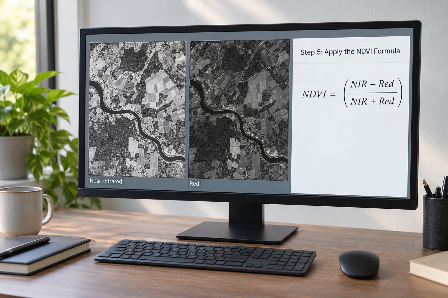
Apply the formula with both bands in reflectance and both in floating point, and guard the denominator so pixels where red and NIR are both zero return no-data rather than a divide-by-zero error. Integer division is the quiet killer here: if the bands stay as 16-bit integers, the division truncates toward zero and your NDVI comes out in steps of one instead of a smooth range.

In the QGIS raster calculator, enter:

("nir@1" - "red@1") / ("nir@1" + "red@1")

QGIS 3.x shows values as floating point by default, but add a denominator check anyway if the output has odd speckling: (("nir@1" + "red@1") > 0) * (("nir@1" - "red@1") / ("nir@1" + "red@1")). Set the output extent to match the input rasters and use a Float32 output data type.

In ArcGIS Pro, open Analysis, then Raster Calculator, and use the NDVI tool directly from the list if you want the built-in parameters, or enter the expression by hand:

Con("NIR_Band5" + "Red_Band4" > 0, Float("NIR_Band5" - "Red_Band4") / ("NIR_Band5" + "Red_Band4"))

The Float cast matters: without it ArcGIS Pro keeps the integer subtraction and you lose precision before the division ever happens.

In Google Earth Engine everything runs in the browser, so no downloads and no projection setup are needed:

var image = ee.Image('COPERNICUS/S2_SR_HARMONIZED/2026-06-15T10-30-00')
  .filterBounds(geometry)
  .first();
var ndvi = image.normalizedDifference(['B8', 'B4']).rename('NDVI');
print(ndvi.reduceRegion({
  reducer: ee.Reducer.mean(),
  geometry: geometry,
  scale: 10
}));

In Python with rasterio and numpy, cast to float first so no-data zeros become NaN, then guard the denominator:

import rasterio
import numpy as np

with rasterio.open('red_band.tif') as src_red, rasterio.open('nir_band.tif') as src_nir:
    red = src_red.read(1).astype('float32')
    nir = src_nir.read(1).astype('float32')
    profile = src_red.profile

denominator = nir + red
ndvi = np.divide(nir - red, denominator,
                  out=np.full_like(nir, np.nan),
                  where=denominator != 0)

The out and where arguments in that divide call are what keep NaN from spreading across pixels that have no valid data.

Step 6: Check the NDVI Results

Valid NDVI falls between -1 and +1. Values below zero generally mean water, bare shadowed ground or cloud, and values above +1 mean something went wrong. Open the result, apply a diverging colour ramp such as RdYlGn with the range fixed at -1 to 1, and look at the pattern.

Then run four checks that catch almost everything:

• Range check. Print the minimum, maximum, mean and standard deviation. A max above 1 or a min below -1 means band mismatch or scaling trouble.
• Denominator check. Sample a pixel where the output is blank and confirm both bands are zero there. If they are not, the mask is doing the work, not the formula.
• Spot comparison. Pick three to five points you know the land cover of and compare the NDVI to what the surface should read. Dense forest high, dry bare soil near zero, water negative.
• Sanity check against experience. For a full, healthy late-season standing crop, a mean around 0.45 is a reasonable expectation. A field mean under 0.40 at a date when neighbouring fields are above it usually means real stress, or a cloud you did not mask.

If you want a firmer validation, download the official Copernicus NDVI 300 m product for the same date, resample it to your grid and compare means over the same polygon. They will not match exactly because of resolution and processing differences, but a difference of more than about 0.05 over the same area means one of the two is wrong.

Step 7: Export and Document the NDVI Raster

Save the result as a GeoTIFF so it opens in any GIS later. In QGIS, use Layer then Save As, choose GeoTIFF, set the data type to Float32 and set the no-data value to -9999. In ArcGIS Pro, use Raster then Export, or the Export Raster tool, and set the output to Float32 with nodata at -9999. In Python, write it with rasterio:

ndvi = np.where(np.isnan(ndvi), -9999, ndvi).astype('float32')
profile.update(dtype='float32', count=1, nodata=-9999, compress='deflate')

with rasterio.open('ndvi.tif', 'w', **profile) as dst:
    dst.write(ndvi, 1)

Then write down the acquisition date, sensor, product level, the exact source band numbers, the formula you applied, any resampling and masking steps, the software and version, and the output pixel size. It takes two minutes and it is the difference between a result you can reproduce a year later and a folder of TIFFs nobody can interpret.

Common Mistakes

Reversed bands in the formula

Writing (Red – NIR) instead of (NIR – Red) flips the sign of every pixel, so healthy vegetation reads strongly negative and water reads positive. The map still looks plausible, which is why this survives review. Check one pixel you know the land cover of: if a vegetated field comes out negative, the terms are swapped.

Integer division truncating the result

Both bands stay 16-bit integers and the division collapses to whole numbers. Fix it by casting both arrays to float32 before the subtraction, or by using the Float function in the ArcGIS raster calculator. The tell is an NDVI map made of a few flat blocks rather than a smooth gradient.

Mismatched pixel grids

The red band comes from one product or resolution and the NIR band from another, so each pixel is paired with the wrong neighbour and the result is spatially scrambled but still statistically normal-looking. Fix it by reprojecting and resampling one band onto the other with a shared extent, cell size and origin before the calculation.

Cloud and shadow contamination

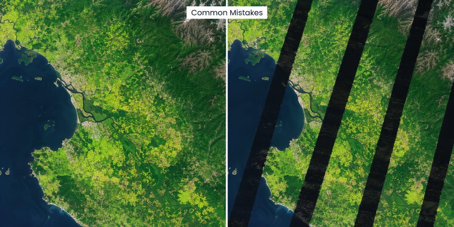
Thin cloud reads as a moderate, misleadingly healthy NDVI and cloud shadow reads as negative, so an unmasked scene invents stress that is not there. Fix it by applying the product’s classification band as a shared mask on both inputs, and re-run on a clearer date if more than a tenth of your area is cloudy.

Unmasked no-data values

No-data pixels are stored as zero, so (0 – 0) / (0 + 0) becomes a divide-by-zero and floods the map with blank or error values. Fix it by casting to float so zeros become NaN and by using the out and where arguments in numpy divide, or the Con guard in ArcGIS.

Values outside the -1 to +1 range

Anything beyond the range means the two inputs are not the same kind of quantity. Most often one band was left as raw scaled integers while the other was converted to reflectance. Fix it by confirming both bands come from the same product level and the same scaling convention.

Tips for Reliable NDVI Results

Use the same product level for every scene in a comparison. Mixing Level-1 and Level-2 across a season introduces offsets that look like vegetation change but are processing differences.

Keep the native resolution of the sensor you chose. Upsampling 30 m Landsat to 10 m does not add detail, it only makes the map look sharper and inflates your area estimates.

Compare dates that are consistent. Same month, similar days apart, similar sun angle, avoids confounding phenology with viewing geometry.

Remember NDVI is a relative indicator. A 0.05 rise matters more in a dry, sparse-canopy setting than in a dense one, and it means nothing at all without a reference date from the same field.

Know where the index stops being useful. Above roughly 0.9, dense canopy saturates and the number stops responding to real differences in biomass. If soil is visible between plants, the red band is picking up soil brightness rather than vegetation. In both cases SAVI or EVI behaves better, and a wetland index like NDWI is the right tool if water fraction is what you are actually mapping.

Frequently Asked Questions

Conclusion

Start by identifying your sensor’s red and near-infrared band numbers and its product level, because every error downstream traces back to getting that pair wrong. Put both bands on one grid, cast them to float, apply (NIR – Red) / (NIR + Red) with a guard on the denominator, then check the result against the -1 to +1 range and against a few pixels whose land cover you know. Only after the validation passes is the map worth interpreting or exporting.