How to Check Normality of Data in SPSS (2026): Easy Steps

To check normality of data in SPSS, open Explore from Analyze > Descriptive Statistics > Explore, move your variable into the Dependent List, then tick Tests of Normality under Statistics and Normality plots with tests under Plots. Read the Sig. column in the output: above .05 means no significant deviation, below .05 means there is one. The whole check takes about two minutes once your data are loaded.

This guide walks through that process step by step, explains what the histogram and Q-Q plot are telling you, and shows you how to report the result in your thesis. It works in IBM SPSS Statistics 26 through 30 and the menu names are the same on Windows and Mac.

Table of Contents

1. 1What You Need Before You Start
2. 2Step-by-Step: How to Check Normality of Data in SPSS
3. 31. Check the Variable and Analysis Assumption
4. 42. Run the Normality Test in SPSS
5. 53. Examine the Histogram and Q-Q Plot in SPSS
6. 64. Apply a Practical Decision Rule
7. 75. Check Skewness and Kurtosis With Z-Scores
8. 86. Report the Result and Choose the Next Step
9. 9Common Mistakes to Avoid
10. 10Frequently Asked Questions
11. 11Should I use the Shapiro-Wilk or Kolmogorov-Smirnov test in SPSS?
12. 12Is a normality-test p-value above .05 proof that my data are normal?
13. 13How many observations are too many for a normality test in SPSS?
14. 14Should I check normality before or after removing outliers?
15. 15What should I do when my SPSS data are not normally distributed?
16. 16Conclusion

What You Need Before You Start

Have these four things settled before you click anything. Most confusion in the output comes from testing the wrong thing, not from running the test badly.

• The variable you are actually testing. Not every variable in your dataset needs a normality check. Only the ones feeding a parametric test.
• The assumption behind your analysis. A t-test or ANOVA assumes each group’s values are roughly normal. Regression and Pearson correlation assume it for the residuals, not for the outcome variable itself.
• Your sample size. It changes how you read the p-value, badly at both ends. Under about 50 cases the tests are unreliable; over 2000 they flag trivial departures.
• A quick outlier look. Graphs > Legacy Dialogues > Boxplot on the same variable. One extreme case can push a perfectly normal-looking variable to Sig. .001.

Also set the measurement level properly in Variable View. A variable still marked nominal will not behave like a continuous measure in the analysis that follows.

Step-by-Step: How to Check Normality of Data in SPSS

1. Check the Variable and Analysis Assumption

Normality is not a property of a dataset. It is a property of the specific values your test will work with. Before running anything, match your planned analysis to the right check.

• Comparing two or more groups (t-test, ANOVA): test each group separately, not the pooled variable. Pooling hides a skewed subgroup behind a balanced other one.
• Running regression or correlation: test the residuals saved from the model, not the raw predictor or outcome.
• Describing a single continuous variable: the overall Explore output is enough.
• Working with 1 to 5 Likert items: single items are ordinal and a normality test on them tells you little. Test the composite score you actually analyse.

If you are unsure which applies, start with the overall check and refine from there.

2. Run the Normality Test in SPSS

Click through in this order:

1. Analyze > Descriptive Statistics > Explore.
2. Select your variable and click the arrow into the Dependent List. Use Factor List only when you are splitting the output by a grouping variable such as gender or condition.
3. Click Statistics. Tick Descriptives and Tests of Normality. Click OK.
4. Click Plots. Tick Histogram and Normality plots with tests. Click OK.
5. Click OK to run.

SPSS prints a Tests of Normality table with one row per variable and two statistic columns: Shapiro-Wilk (W) and Kolmogorov-Smirnov (D), each with a Sig. column. There is no separate normality command to install. Users on SPSS 29 or 30 who go looking for an extension are looking for something that already exists in this dialog.

If you prefer reproducible output, the syntax is:

EXAMINE VARIABLES=yourvar
  /STATISTICS DESCRIPTIVES KURTOSIS SKEW
  /PLOT=NPPLOT /PLOT=HISTOGRAM
  /MISSING LISTWISE.

Run it from the syntax window and the output is identical, which matters when your supervisor asks for a reproducible analysis appendix.

One thing trips people up here. If you put three variables into the Dependent List and the Shapiro-Wilk value for one of them changes compared with when it ran alone, that is expected behaviour in the Explore output rather than a bug. Run each variable in its own pass when you need stable, reportable values.

3. Examine the Histogram and Q-Q Plot in SPSS

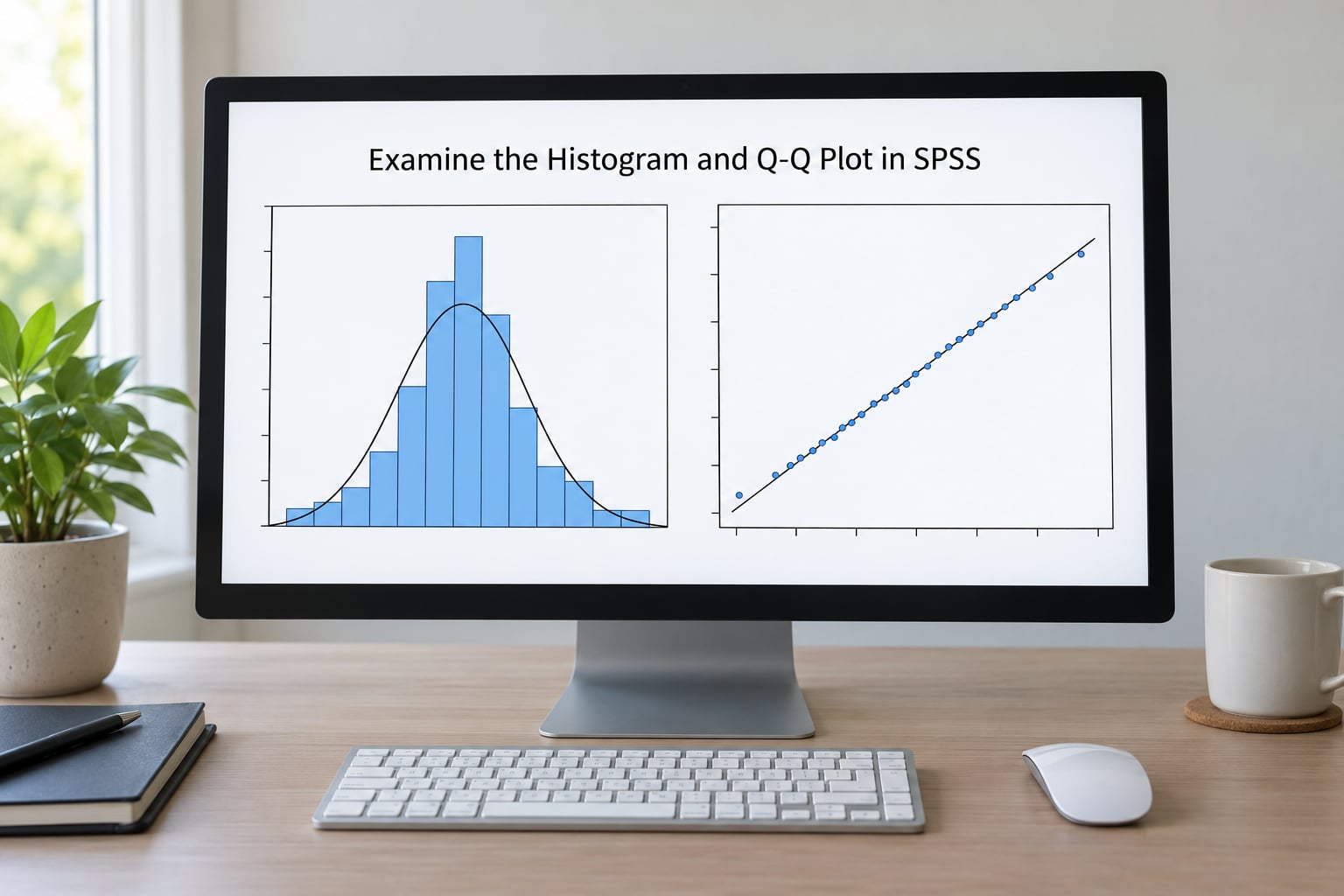
The numeric test only tells you whether a departure is detectable. The pictures tell you how big it is and where it comes from.

Histogram. Look for a single peak near the centre with tails that fall away roughly symmetrically, and compare the bar shape to the overlaid normal curve. A one-sided tail stretching out, a flat top, or a visible pile of values at one end all indicate skewness. That is fine to a point.

Q-Q plot. Each dot plots an observed value against the value a normal distribution would predict. Points sitting on the diagonal reference line mean a good normal fit. Points in a smooth curve, or a couple of points far off the ends, mean the tails or the extremes diverge from normal.

Detrended Normal Q-Q Plot. SPSS produces this second plot when you tick the box, and it removes the overall trend so you see only deviation from the line. It makes a subtle departure obvious when the standard plot looks fine.

When the histogram looks slightly lopsided but the Q-Q points stay near the line, that is mild skewness. You can usually proceed.

4. Apply a Practical Decision Rule

Read the Sig. value as a p-value, not as a verdict. The null hypothesis is that the values come from a normal distribution, so a small Sig. is evidence against normality, not evidence of it.

• Sig. above .05: you failed to reject normality. That is permission to continue with a parametric test, not proof the data are perfectly normal.
• Sig. below .05: there is a statistically detectable departure. Look at the histogram and Q-Q plot to see whether it is mild or severe before reacting.
• Sig. .049 or similar: a threshold is not a cliff. A skewness Z of 1.2 with a near-linear Q-Q plot is not a problem in practice.

Sample size does most of the damage here. Past roughly 2000 cases, tiny departures that will never affect your results still produce Sig. below .05. For those datasets, judge normality on the skewness and kurtosis values and the Q-Q plot, and mention the deviation in your write-up instead of swapping tests.

5. Check Skewness and Kurtosis With Z-Scores

This is the second opinion most supervisors want to see. Go to Analyze > Descriptive Statistics > Descriptives, click Options, and tick both Kurtosis and Skewness under the Distribution group.

The output table gives you raw skewness and kurtosis alongside standardized Z-scores, which are the raw values divided by their standard errors. The Z-scores tell you how far each is from zero relative to sampling noise, which is why they behave better in large samples than the raw numbers.

A common academic rule is that Z values should sit between -1.98 and +1.98 for a strict fit, and inside -3 to +3 for a looser one used with large samples. Judge each separately. Skewness between -1 and +1 with kurtosis between -2 and +2 is a widely accepted practical range, and most t-tests and ANOVAs survive it comfortably.

6. Report the Result and Choose the Next Step

When the result is acceptable, a standard APA line reads:

A Shapiro-Wilk test confirmed that the distribution of scores was not significantly different from normal, W = 0.98, p = .21.

When it is not:

Scores departed significantly from normality, Shapiro-Wilk W = 0.94, p = .002. A Mann-Whitney U test was therefore used in place of the independent-samples t-test.

For group comparisons, add the group split. Select Data > Split File by your grouping variable first, then run Explore again so each group gets its own row, histogram and Q-Q plot. The same rule applies inside Compare Means > Independent-Samples T Test, which prints a per-group table when you click Options.

If the data fail, you have four options in order of preference:

1. Check the outliers first. One extreme case often explains the whole departure. Boxplot, then decide whether that case is an error or a genuine observation.
2. Switch to the robust equivalent. Independent t-test becomes Mann-Whitney U; one-way ANOVA becomes Kruskal-Wallis; Pearson becomes Spearman.
3. Transform the data. Transform > Compute Variable handles log and square root functions. A strong right skew on income or response time often fixes itself this way.
4. Keep the parametric test. With balanced groups and sample sizes above 30, t-tests and ANOVAs are quite tolerant of mild non-normality. Say so in your write-up.

Common Mistakes to Avoid

• Relying on one test. A single Sig. value is one signal out of four. Combine the p-value, the Z-scores, the histogram and the Q-Q plot before deciding.
• Treating Sig. above .05 as proof. Failing to reject means the test found nothing, which is not the same as confirming a normal distribution. This is the most common misreading in student write-ups.
• Testing raw data when the assumption concerns residuals. In regression and correlation, save the residuals and run Explore on them instead.
• Running tests on very large samples without thinking. Above 2000 cases, expect every variable to come back significant and use the practical measures instead.
• Looking at skewness or kurtosis on its own. A value of 2.5 means different things with a small Z and a large one.
• Deleting real cases to tidy the output. Dropping observations purely to make a test pass is data misuse. Remove only cases you can justify as errors, and document it.
• Transforming with no reason. A square root of a negative value, or a log of a score with zeros, produces nonsense. Transformation changes interpretation, so justify it in your method section.
• Testing a Likert item as if it were continuous. Test the composite score instead.

Frequently Asked Questions

Conclusion

Run Explore, then read four things together: the Shapiro-Wilk Sig. value, the skewness and kurtosis Z-scores, the histogram shape and the Q-Q plot. Judge each against your sample size, check outliers before transforming anything, and report all of it in your write-up rather than a single number. Whichever way the result lands, the analysis is defensible because you looked properly. IBM SPSS Statistics keeps the same dialogs across versions, so a walkthrough built on 2026 still applies to the release you have open.