
To analyze panel data for a thesis, you reshape your data into long format with one row per entity per period, declare it as a panel, run descriptive and balance checks, then estimate fixed effects, random effects or pooled OLS and test the assumptions behind your choice. The whole workflow takes a few hours the first time and about twenty minutes once you have the commands saved.
Panel data means the same units, such as people, firms, regions or countries, are observed repeatedly across several periods. That repetition is the point. It lets you separate what changes inside a unit from what was always different about it, and it removes a lot of the omitted variable worry that makes a single cross-section fragile.
The order below is the one I would follow, and it is the order that keeps a supervisor from sending your draft back. Data shape first, description second, model choice third, diagnostics fourth, write-up last.
Table of Contents
- 1What You Need
- 2The panel structure
- 3The two keys
- 4Variables with a reason
- 5Balanced or unbalanced panel
- 6Software
- 7How many units and periods you need
- 8Where the data usually comes from
- 9Step-by-Step
- 101. Define the research question and unit of analysis
- 112. Check and prepare the panel dataset
- 123. Explore the data with panel summaries
- 134. Choose the appropriate panel model
- 145. How to Analyze Panel Data in Stata and R
- 156. Test panel-data assumptions
- 167. Run sensitivity and robustness checks
- 178. Interpret and report the results
- 18Common mistakes that get flagged in panel analysis
- 19Frequently Asked Questions
- 20What is panel data?
- 21When should I use fixed effects instead of random effects?
- 22What are year fixed effects and why would I add them?
- 23Why does my fixed effects model drop my gender or education variable?
- 24Should I use Stata or R for panel data analysis?
- 25Can I analyze panel data when some entities are missing periods?
- 26Conclusion
What You Need
Before you run anything, you need four things in place: a dataset that is already in long format, an entity identifier, a time identifier, and a clear statement of your outcome variable. Everything else in this guide assumes those four exist.
The panel structure
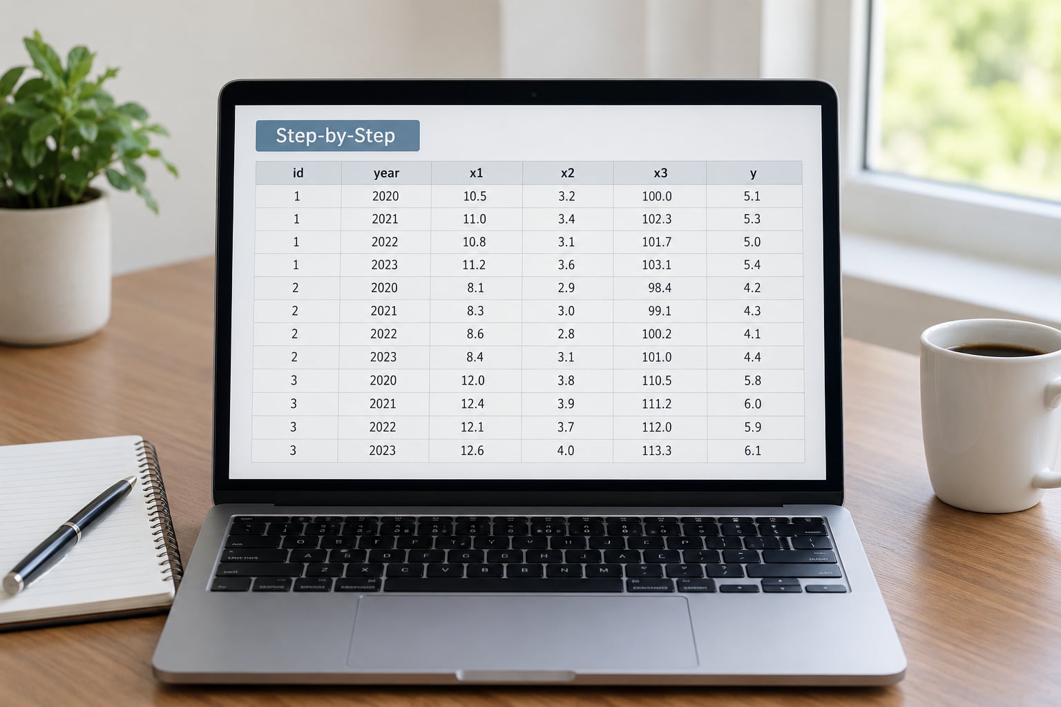
Long format means one row per unit per period. If you follow 500 workers over eight years, you have 4,000 rows, not eight. Wide format, where each wave is its own variable, has to be reshaped before any panel command will work.
Most survey downloads arrive wide, and this is the step where new users get stuck. Forum threads on r/stata and Statalist are full of people whose variables simply will not appear because the data never declared a time key.
The two keys
You need one variable that identifies the unit and one that identifies the time period. Person ID and year, firm ID and fiscal year, country ISO code and calendar year. Each unit-period pair should be unique, and if it is not, your merge produced duplicates rather than a panel.
Variables with a reason
An outcome variable measured on the same scale across periods, one or more explanatory variables that actually vary within units, and a short list of control variables your theory supports. Forum advice on r/econometrics is consistent on this point: start from the literature and your theoretical relationship, not from the hundred variables the survey happens to contain.
Balanced or unbalanced panel
A balanced panel has every unit observed in every period. An unbalanced panel has gaps, usually from attrition or item non-response. Both are usable. What you cannot do is silently report one sample size when your estimation used another.
Software
Stata and R handle everything below. Python users work with linearmodels or PanelOLS from linearmodels, and some institutions teach SPSS MIXED syntax for the same models. SPSS exists in plenty of departments, but the panel diagnostics are thinnest there, and Hausman tests are awkward outside Stata.
The four packages produce the same point estimates for the same model. What differs is how much work the diagnostics take, so pick based on what you will need later rather than what is installed on your laptop.
| Package | Declare the panel | Fixed effects | Diagnostics |
|---|---|---|---|
| Stata | xtset id time | xtreg y x, fe | xtserial, xttest0, hausman built in |
| R (fixest) | Implicit in the formula | feols(y ~ x | id + year) | Built-in checks, small model matrix |
| R (plm) | Implicit in plm() | model = “within” | plmtest, pbgtest, pcdtest |
| Python (linearmodels) | PanelOLS | entity_effects=True | Manual, mostly |
| SPSS | Define id and time | MIXED syntax | Limited for panel-specific tests |
How many units and periods you need
There is no magic number, but there are floors. You want enough units that clustered standard errors behave, so 30 units is about the minimum and 50 or more is comfortable. Periods matter less for a static panel than people expect, since your variation comes mostly from cross-sectional units.
Large N with small T is the classic setup, and it is where dynamic panel estimators earn their place. Small N with large T is fine for fixed effects but thin for anything requiring cluster-robust inference. If you have only two periods, first differences or a fixed effects model are the honest choices.
Where the data usually comes from
Household panels such as BHPS, Understanding Society, PSID and HRS give you people repeated over many waves. Country-level work usually draws on the World Development Indicators or Eurostat. Whatever the source, download the codebook before the data file and write down how each variable is defined across waves, because definitions often shift mid-panel.
Step-by-Step
1. Define the research question and unit of analysis
Write the relationship you want to estimate before you touch the data. Outcome, main explanatory variables, the comparison you are making, and the direction you expect.
The unit of analysis is the thing that repeats. Individuals, firms, regions. Getting this wrong is the most common reason a thesis model does not behave the way the student predicted, because the software was counting the wrong rows.
How to tell it worked: you can state your estimand in one sentence, for example the effect of training hours on hourly wage within the same worker over time.
2. Check and prepare the panel dataset
Reshape to long format, check for duplicate unit-period keys, confirm variable types, then declare the panel structure so the software knows what it is looking at.
In Stata, reshape long income hours age, i(person) j(year) turns eight wide year variables into one long column. Then xtset person year declares the panel, and xtdescribe tells you what the software thinks it has.
In R with the reshape2 route, reshape(df, idvar="person", varying=list(2:9), timevar="year", direction="long") does the same job, followed by panel_plm <- plm(y ~ x + controls, data = df, model = "within").
Check balance directly. In Stata, xtdescribe gives you the number of units, the minimum and maximum periods, and the count of gaps. In R, table(df$person) shows how many periods each unit contributes.
How to tell it worked: xtset returns without an error, the gap count matches your expectations, and no unit-period pair appears twice. If isid person year in R throws a duplicate message, fix the merge before going any further.
3. Explore the data with panel summaries
Compute descriptive statistics, look at how the outcome moves over time, and separate within-unit variation from between-unit variation. That last split decides which effects are even identifiable in your data.
Within variation is the movement in a variable inside a single unit over time. Between variation is the difference in the average level across units. A variable with no within variation, such as a person’s sex assigned at birth or their country of birth, cannot be estimated in a fixed effects model because nothing inside the unit ever changes it.
Stata gives you sum income hours age, detail and xtsum income hours age for overall, within and between spread. R’s fixest package does the same through summary(feols(y ~ x | id + year, data = df)).
Plot the outcome by unit over time and check for outliers before estimating anything. Forum users report that a handful of extreme within-unit observations can swing a fixed effects estimate badly, and that trimming or winsorising after seeing the plots is routine practice.
How to tell it worked: you can say, in a sentence, which of your variables carry meaningful within-unit variation. That sentence becomes the justification for your model choice later.
4. Choose the appropriate panel model
Choose based on your research design and what the data look like, not on which estimator gives the prettiest table. Pooled OLS ignores all heterogeneity, fixed effects absorbs everything time-invariant about a unit, random effects assumes that heterogeneity is unrelated to your regressors, and dynamic panel models handle persistence when T is small.
| Model | Key assumption | Estimates time-invariant variables? | Use it when |
|---|---|---|---|
| Pooled OLS | No unit or time heterogeneity | Yes | Benchmark only, reported as model 1 |
| Fixed effects (within) | Unit effects uncorrelated with regressors | No | You care about within-unit change and cannot rule out correlation |
| Random effects (GLS) | Unit effects uncorrelated with regressors | Yes | Units are a sample from a larger population and correlation is implausible |
| First differences | Similar to FE, different weights | No | Two periods only, or you want a differencing interpretation |
| Dynamic panel (GMM) | Lagged dependent variable, valid instruments | Partly | Large N, small T, strong persistence in the outcome |
The decision rule in one line: use fixed effects when your explanatory variables vary within units and correlation between unobserved unit characteristics and those variables is plausible. Use random effects only when you can defend the opposite, which is a strong claim for most thesis data.
How to tell it worked: your model choice can be traced to a paragraph of theory plus a sentence about within-unit variation. If it rests only on a test result, examiners will push back.
5. How to Analyze Panel Data in Stata and R
Estimate the specification you chose, add the controls your theory supports, and set standard errors appropriate to the sampling design. The command is short; the thinking behind the controls is the work.
* Stata: pooled, then fixed, then random
xtset person year
reg income hours age i.year, cluster(person)
xtreg income hours age i.year, fe vce(cluster person)
xtreg income hours age i.year, re vce(cluster person)

* Random effects Hausman test, run right after the RE model
hausman fe_model re_model, sigmamore
# R with fixest: one line per estimator, clustered SE throughout
library(fixest)
m1 <- feols(income ~ hours + age, data = df, cluster = ~person)
m2 <- feols(income ~ hours + age | person + year, data = df, cluster = ~person)
m3 <- feols(income ~ hours + age | year, data = df, cluster = ~person)

# R with plm, including the Hausman test
library(plm)
p1 <- plm(income ~ hours + age + factor(year), data = df, model = "pooling")
p2 <- plm(income ~ hours + age + factor(year), data = df, model = "within")
p3 <- plm(income ~ hours + age + factor(year), data = df, model = "random")
plmtest(p2, p3)
Cluster standard errors on the entity identifier. They are the standard answer for panels, because they allow correlation within a unit over time and across observations that share that unit. Robust, non-clustered errors treat 4,000 rows as 4,000 independent observations, which they are not.
How to tell it worked: the number of clusters is large enough for the inference to mean something, usually 30 or more units, and your coefficient signs match what the descriptive analysis showed.
6. Test panel-data assumptions
Panel models assume more than ordinary least squares does. Check serial correlation, heteroskedasticity and cross-sectional dependence, and run the Hausman test where the fixed versus random effects decision is in play.
The Hausman test compares fixed and random effects estimates under the null that the unit effects are uncorrelated with the regressors. Rejecting the null supports fixed effects. Rejecting it is the normal expectation and not a problem.
Students get this backwards often enough to say it plainly: a non-significant Hausman test does not prove random effects are correct. The test has low power in small samples, and using the sigmamore option in Stata gives the more reliable version. If the two models disagree, report both and explain why you chose the more conservative estimator.
Run the rest of the checks with these:
| What you are testing | Stata | R | If it fails |
|---|---|---|---|
| Serial correlation in panel residuals | xtserial | pbgtest in plm | Cluster by entity, or use Driscoll-Kraay with vce |
| Heteroskedasticity | xttest0 | plmtest | Clustered standard errors usually solve it |
| Cross-sectional dependence | Pesaran CD or xtreg with Driscoll-Kraay | plm::pcdtest | Two-way clustered errors or a wild bootstrap |
| Random effects consistency | hausman, sigmamore | plmtest(p2, p3) | Stay with fixed effects and say why |
| Multicollinearity | vif, reg | car::vif | Drop or combine overlapping controls |
Statistical significance and practical importance are separate questions. A coefficient of 0.4 on an outcome measured in thousands can be trivial, and a coefficient with a p-value of 0.08 can still be the largest effect in your table. Say which one you are dealing with.
How to tell it worked: you have a table or a short paragraph listing each test, its statistic, and what you did about it. A thesis that reports no diagnostics at all invites the question it should have answered.
7. Run sensitivity and robustness checks
Re-estimate the preferred model with sensible variations and see whether the main result moves. Supervisors ask for this because a result that only holds in one specification was fragile to begin with.
The standard set: pooled OLS and fixed effects side by side, then with year fixed effects added, then with the dependent variable as a log, then on a balanced subsample, then with a lagged dependent variable if your theory implies persistence. Replace any variable with a plausible alternative measure where one exists.
If you have a dynamic relationship and few time periods, check whether GMM is worth reporting alongside the static model. Arellano-Bond and Blundell-Bond estimators exist for exactly this case, with the xtabond2 command in Stata or plm::pgmm in R.
How to tell it worked: the coefficient on your main variable keeps its sign and rough magnitude across specifications. If it flips, you have a finding about heterogeneity to explain, not a failure to hide.
8. Interpret and report the results
Turn output into prose a reader can follow. State what a one-unit change in the explanatory variable does to the outcome, name the unit of the outcome, give the confidence interval alongside the p-value, and stay inside what your design supports.
Fixed effects coefficients are within-unit effects: the change in the outcome associated with a change in the regressor for the same unit, holding other included variables constant. Random effects coefficients blend within and between variation, which means a reader cannot interpret them as a pure within effect without further work.
Fixed effects models also report three R-squared values. The within R-squared measures how much of the movement inside units is explained, and the between R-squared measures how much of the differences across unit averages is explained. Report the one that matches your estimand and name it explicitly.
A results table usually carries a dependent variable row, one row per explanatory variable with coefficient and standard error in parentheses, a row for constants, rows for fixed effects, time effects and clustering, and the observation and unit counts underneath.
How to tell it worked: a reader who has never seen your data can tell what the main finding is, how large it is, and how confident you are in it. Avoid causal language that the design cannot carry, such as saying a treatment caused an outcome change in a simple observational panel.
Common mistakes that get flagged in panel analysis
These come up repeatedly in thesis feedback and forum threads, and each one has a direct correction.
- Running the analysis in wide format. Fix: reshape to long with an entity and time key, then declare the panel before estimating anything.
- Reporting ordinary standard errors. Fix: cluster on the entity identifier, or use Driscoll-Kraay where cross-sectional dependence is present.
- Treating missing units as absent without saying so. Fix: report how many units drop at each stage and why, and state whether the panel is balanced.
- Choosing random effects because the Hausman test was insignificant. Fix: treat the test as one piece of evidence and justify the estimator from the research design.
- Using the two-way model and commenting only on the coefficient. Fix: explain that year effects absorb shocks common to every unit in that period.
- Overstating causality. Fix: match the wording to the design, and name the identifying assumption you rely on.
- Reporting a final model with no diagnostics. Fix: attach the test table from step 6 to the appendix and reference it in the text.
One more worth knowing: when fixed effects drop a variable silently, it is almost always because the variable is time-invariant within your sample. That is a property of the estimator, not a bug in your data.
Frequently Asked Questions
What is panel data?
Panel data follows the same units, such as people, firms, regions or countries, across multiple time periods. Because each unit is observed more than once, you can separate change within a unit from stable differences between units, and you can absorb characteristics that never change over time. A panel is balanced when every unit appears in every period, and unbalanced when some units have gaps.
When should I use fixed effects instead of random effects?
Use fixed effects when your explanatory variables vary within units over time and you cannot rule out a correlation between unobserved unit characteristics and those variables. Use random effects only when the unit effects are plausibly uncorrelated with your regressors, such as when units are a random sample from a much larger population. When in doubt, fixed effects is the more conservative choice and is easier to defend in a thesis.
What are year fixed effects and why would I add them?
Year fixed effects add one dummy variable for each time period, capturing every shock that hit all units in that year at once, such as a recession, a policy change or a pandemic. Adding them absorbs common time variation, so your remaining coefficients reflect within-unit differences rather than shared events. In Stata add i.year to an xtreg model, and in R add factor(year) to the formula.
Why does my fixed effects model drop my gender or education variable?
A fixed effects model can only estimate variables that change within a unit over time. Gender, ethnicity, country of birth and other characteristics fixed for the life of the unit have no within-unit variation, so the estimator cannot separate their effect from the unit intercept and drops them. That is a feature of the estimator, not a data problem. Use correlated random effects, or estimate those variables with a pooled or random effects model.
Should I use Stata or R for panel data analysis?
Both handle panel work well and produce the same estimates. Stata has the shortest path for panel diagnostics, with xtset, xtreg, xtserial, xttest0 and the hausman command built in, which is why it dominates economics departments. R gives you more modelling options through plm, fixest and PanelOLS, plus easy graphics. Pick the one your supervisor reads, and learn the equivalent commands in the other later.
Can I analyze panel data when some entities are missing periods?
Yes. An unbalanced panel is normal in survey and administrative data, and most panel estimators handle it directly, though some theory assumes balance. Report how many units drop at each stage, state plainly that the panel is unbalanced, and check whether the missing units differ systematically from the rest. As a robustness check, re-estimate on the balanced subsample and see whether the main result holds.
Conclusion
Start with the data, not the model. Write down your unit of analysis, reshape to long format, declare the panel, and run a balance check before you think about estimators.
Then pick the model your design supports, not the one a test points at, and remember that to analyze panel data for a thesis properly means showing the diagnostics and the robustness checks alongside the main table. A supervisor who can see your work is far easier to convince than one who only sees a final coefficient.