How to Analyze Pre and Post Test Data: An Easy SPSS Guide (2026)

To analyze pre and post test data, match each participant’s pretest score with their post-test score, compute the difference for every pair, then test whether the average difference is reliably different from zero. Use a paired-samples t-test when the differences are roughly normal, and the Wilcoxon signed-rank test when they are not.

That is the whole logic. Each person is their own comparison, so the analysis is about within-person change rather than a difference between two groups of people.

I have watched students lose hours on this one mistake: running an independent-samples t-test on two columns of pre and post scores. It runs, it produces a p-value, and it answers the wrong question. Once the pairing is dropped, you inflate the standard errors, throw away the statistical power that the pairing gave you, and quietly change what your study is about.

Below is the workflow I walk students through, with the exact menu paths, the assumption checks people skip, and a reporting line you can paste straight into your paper. Last reviewed for 2026.

Table of Contents

1. 1What You Need Before You Analyze Anything
2. 2Step-by-Step: How to Analyze Pre and Post Test Data
3. 3Step 1: Identify the Paired Study Design
4. 4Step 2: Prepare and Inspect the Data
5. 5Step 3: Choose the Appropriate Statistical Test
6. 6How to Analyze Pre and Post Test Data in SPSS
7. 7How to Run the Analysis in R or Stata
8. 8Step 4: Interpret the Results
9. 9Step 5: Report the Findings
10. 10Common Mistakes in Pre and Post Analysis
11. 11Common Mistakes and Quick Fixes
12. 12Your post-test has fewer rows than your pre-test
13. 13You cannot link the two surveys to the same person
14. 14Your data are in two columns and you need long format
15. 15You have missing scores in both waves
16. 16Your participants sit inside classrooms or teams
17. 17Your result is not significant
18. 18Post-test-only questions
19. 19Frequently Asked Questions
20. 20How do you analyze pretest-posttest data?
21. 21Which statistical test should I use for pre and post test data from the same participants?
22. 22Why use Wilcoxon instead of t-test for pre and post data?
23. 23When should you do a paired t-test rather than repeated measures ANOVA?
24. 24What is the best test to use for analyzing Likert scale pre and post data?
25. 25Can I use ANOVA to compare pre and post scores?
26. 26Conclusion: Start With the Research Design

What You Need Before You Analyze Anything

Five things have to be true before any test is worth running, and all five are decided by design, not by software.

1. Paired observations. The pre and post scores belong to the same participants. Not two groups of similar people, the same individuals measured twice.
2. A participant identifier. Some column that ties row 14 in the pretest file to row 14 in the post-test file. Without it there is no analysis at all, just arithmetic.
3. One row per participant, two score columns. Wide format: id, pre_score, post_score. Every paired test expects this layout.
4. Software with a paired routine. SPSS, R, Stata, jamovi, JASP and even Excel all have one. Free tools are fine for this.
5. A measurement scale decision. Interval-style scores that support means and standard deviations, or ordinal items like a 1-to-5 Likert scale where the median is the honest summary.

One more piece of paperwork matters more than most people expect: what happens to participants who only completed one of the two waves. Decide the rule before you look at the scores. A paired test silently drops incomplete pairs, so 40 pretests and 32 post-tests from the same people leaves you with 32 pairs and a smaller sample than the raw counts suggest.

Step-by-Step: How to Analyze Pre and Post Test Data

Step 1: Identify the Paired Study Design

You have a within-subjects design with one factor of time at two levels. That single fact rules out a long list of tests and picks the family you work in: related-samples tests for one outcome, repeated-measures methods when you have more than one outcome or more than two time points, and mixed models when participants nest inside classrooms, teams or sites.

Pre/post data is only paired if the same people supplied both scores. If your pre survey went to one class and the post survey to a different class, you do not have paired data. You have two independent samples that happen to sit on the same timeline, and the honest test is an independent-samples one.

Matched-pairs designs also appear when pairs are formed rather than measured twice: twins, sibling pairs, a person and their matched control, or before-and-after readings on the same machine. The analysis is identical. The pairing comes from how the pairs were built, not from the word “pre.”

Step 2: Prepare and Inspect the Data

Get the data into one row per participant with a stable ID, then look at it before you test it. Three checks catch most problems.

Check the pairing first. Sort by ID and scan the pre and post columns side by side. IDs that repeat, IDs missing from one wave, or the same ID appearing twice are all fixable now and expensive later.

Check the missing values. In SPSS, run Analyze > Descriptive Statistics > Frequencies and inspect the missing counts for each variable. Count how many participants have both a pre and a post score, because that number is your real n. Report that n, not the pretest headcount.

Create a difference score. In SPSS, Transform > Compute Variable, name it difference, and enter post_score - pre_score. In R, d <- df$post_score - df$pre_score. Getting an explicit difference column makes every later check easier, and it is the column you plot.

Descriptives come next. Report the mean and standard deviation for pre, for post, and for the differences, along with the mean difference itself and a 95 percent confidence interval. Add a paired line chart: pre means on the left, post means on the right, one line per participant. Outliers show up as lines that move in the opposite direction to everyone else, and you want to know about them before the test, not after.

Wide format works fine for the paired tests themselves. You will need long format if you later run a repeated-measures ANOVA or a mixed model, where the structure is id, time and score, with each participant appearing twice.

Step 3: Choose the Appropriate Statistical Test

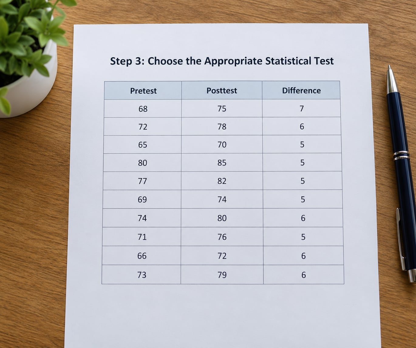
One question decides it: are the differences roughly normally distributed? Not the raw pre scores and not the raw post scores. The differences.

This trips people up constantly. A pretest distribution can be badly skewed and still give you a valid paired t-test, because a skewed pre and a similarly skewed post cancel out in the difference column. Always inspect the difference scores directly, with a histogram, a Q-Q plot, or a Shapiro-Wilk test on the difference variable.

Which test for pre and post test data

Situation	Test to use	Key assumption	Effect size to report
Continuous scores, differences roughly normal	Paired-samples t-test	Differences approximately normal; pairs independent of each other	Cohen’s d (within-subjects form) with 95% CI
Ordinal Likert items or skewed differences	Wilcoxon signed-rank test	Differences symmetric in distribution; at least ordinal measurement	Rank-biserial correlation, Hodges-Lehmann pseudo-median
Differences badly skewed with many ties or zeros	Sign test	Only the direction of change, nothing about magnitude	Proportion of participants who improved
More than two time points, or two outcomes	Repeated-measures ANOVA	Sphericity for three or more levels	Partial eta squared, Greenhouse-Geisser corrected df
Participants nested in groups or sites	Mixed-effects model (linear mixed model)	Random effects structure matched to the sampling design	Fixed-effect coefficient with CI
Nominal outcome, same people, both waves	McNemar’s test	Two categories only; discordant pairs drive the test	Odds ratio of discordant pairs
Post-test-only questions	Descriptive statistics	None, there is no pre value to pair against	Percentages, counts, confidence interval

Two notes on the table. A paired t-test is the default because it is more powerful than its rank-based cousin when the differences are symmetric, roughly 95 percent as efficient under normality. The Wilcoxon signed-rank test earns its place when symmetry fails, when the measurement scale is genuinely ordinal, or when an outlier is inflating the mean difference. And the sign test ignores magnitude entirely, which makes it blunt but hard to break.

How to Analyze Pre and Post Test Data in SPSS

For the paired-samples t-test: Analyze > Compare Means > Paired-Samples T Test. Put the pretest variable in the first box and the post-test variable in the second, in that order. SPSS subtracts the first from the second, so a positive mean difference means improvement when higher scores are better.

Tick Paired Differences and the statistics you want: Descriptives, 95% Confidence Interval, Effect size, and Cohen’s d. Leave Correlation on if you like, since the pre-post correlation itself is worth knowing. Click OK and read the Output window.

The block that matters sits in the Paired Samples Statistics table: mean, standard deviation, standard error of the mean and the correlation for each wave, plus the mean difference, its standard deviation, its standard error, and the 95 percent confidence interval. The Paired Samples Test table gives you t, its degrees of freedom (n minus 1 for the pairs actually used) and a two-tailed Sig. value, which is your p-value.

For the nonparametric route: Analyze > Nonparametric Tests > Legacy Dialogs > 2 Related Samples. Choose Wilcoxon under the Test for, put pre in box 1 and post in box 2, and tick the Z row in the Options box to get the standardized test statistic. The output reports the negative and positive ranks, the sums of ranks for each group, and Z. Older versions of SPSS call the same thing 2 Related Samples directly under the Nonparametric menu.

To check the assumption, run Analyze > Descriptive Statistics > Explore with the difference variable in the Dependent List and press Plots. The histogram plus the normal Q-Q plot is the fastest visual read you will get, and Shapiro-Wilk gives you a number to report if your supervisor asks for one.

How to Run the Analysis in R or Stata

In R the paired t-test is one call with paired = TRUE:

dat <- read.csv("prepost.csv")
res <- t.test(dat$post_score, dat$pre_score, paired = TRUE)
res
res$conf.int
sd(dat$post_score - dat$pre_score)

The Wilcoxon version is wilcox.test(dat$post_score, dat$pre_score, paired = TRUE, exact = FALSE). Add exact = FALSE when you have ties or a sample past about 50 pairs, where the exact distribution is slow and the normal approximation is fine. For effect size, the effsize package’s cohen.d function returns the rank-biserial correlation.

Stata reads the same wide file directly. paired t post_score pre_score gives you the t-test with its confidence interval, and ranksum post_score pre_score runs the Wilcoxon signed-rank test. If your data are still wide, reshape long score, i(id) j(time) turns them into the two-column-per-row layout that anova time and mixed score || id: expect.

Excel does it too. Data > Data Analysis > t-Test: Paired Two Sample for Means, with the pre column in range 1 and the post column in range 2. Excel gives you the test and the two-tailed probability but stops short of effect size and confidence intervals, so I use it for a quick look and rerun it properly afterward.

Step 4: Interpret the Results

Read five numbers, in this order.

Mean difference. The average change from pre to post, with a 95 percent confidence interval. Report the interval every time. A mean improvement of 8 points with a confidence interval running from 2 to 14 tells a completely different story from the same 8 points with an interval from minus 6 to 22.

The test statistic and degrees of freedom. t with df equal to one less than the number of complete pairs. A t of 1.4 means the mean difference is a weak signal against its own standard error.

The p-value. Below .05 is the usual convention, but p does not measure size or importance. It tells you how surprising the observed change would be under no real effect. With a large enough sample, a change too small to matter in practice still reaches significance.

Effect size. Cohen’s d in the within-subjects form is the standardized mean difference, usually around 0.2 for a small effect, 0.5 for a medium one and 0.8 for a large one. For Wilcoxon, report the rank-biserial correlation or the Hodges-Lehmann pseudo-median, which is the median of all pairwise differences.

Number of complete pairs. Not your pretest headcount. If the pairing dropped people, say so and explain why.

A non-significant result is not a failed study. It means the data do not support a change claim at your sample size, and reporting it honestly with the confidence interval is far more credible than rerunning tests until something turns significant. There is an interesting power fact hiding here too: the paired test is more powerful than the independent one, because it removes between-person variation from the comparison.

Step 5: Report the Findings

APA 7 wants the test, the statistics, the effect size and the conclusion, in that order.

Paired t-test. A pre-post test showed that knowledge scores increased from a mean of 54.2 (SD = 8.6) at pretest to 66.9 (SD = 7.1) at post-test, a mean increase of 12.7 points, 95% CI [9.8, 15.6], t(31) = 9.44, p < .001, d = 1.68.

Wilcoxon signed-rank test. Satisfaction ratings increased significantly from pre-test to post-test (median 3 to 4), Wilcoxon W = 142.5, Z = -3.21, p = .001, rank-biserial r = .46.

With a control group. Students in the intervention group improved more than the comparison group, and the Time × Group interaction was significant, F(1, 58) = 6.14, p = .017, partial η² = .096.

Then state the conclusion in one plain sentence, and be careful with the verb. Scores changed. Scores increased significantly. A claim that the intervention caused the change needs a comparison group, because without one you cannot rule out maturation, regression to the mean, testing familiarity or a cohort effect. Keep that sentence within what your design can actually support, and let the confidence interval do the rest of the work.

If you do have a control group, the stronger designs are ANCOVA with the post-test as the outcome and the pre-test as a covariate, or difference-in-differences, which compares the change in the intervention group with the change in the control group. Both use the pre-test as a baseline adjustment and give you a much more defensible causal claim than a one-group before-and-after comparison.

Common Mistakes in Pre and Post Analysis

These are the errors I see most, in roughly the order they happen.

Using an independent-samples test on paired data. Two columns and an independent t-test. Fix: use Paired-Samples T Test, or paired = TRUE in R.

Checking normality of the raw scores instead of the differences. A histogram of the pretest column tells you nothing about the assumption. Fix: plot and test the difference column.

Choosing the test after seeing the p-value. Run both, report the one that looks better. Fix: write the test and its assumption check into your analysis plan before you run anything.

Running one paired test per Likert item. Twenty items means twenty tests and a false positive rate well above 5 percent. Fix: build a scale score, check its reliability with Cronbach’s alpha or McDonald’s omega, and test the total. If item-level change matters, correct with Holm or Bonferroni and say so.

Forgetting that a single item is ordinal. A 1-to-5 Likert item is not an interval variable, so a t-test on it is hard to defend even with a large sample. Fix: either sum items into a scale or use the rank-based test for the item alone.

Leaving outliers unchecked. One participant who gained 200 points drags the mean difference and the standard error with it. Fix: inspect the difference scores with a boxplot, run the test with and without the case, and report the sensitivity check.

Ignoring the sample size. With seven complete pairs, normality testing has almost no power and no test is well calibrated. Fix: report the small n, lean on the confidence interval, and consider an exact or permutation version of the test.

Pasting raw software tables into the paper. Fix: write the APA sentence yourself and cite the output tables as an appendix.

Common Mistakes and Quick Fixes

Here is the same ground in problem-and-fix form, for when a specific error is what brought you here.

Your post-test has fewer rows than your pre-test

Count complete pairs before anything else, because SPSS decides your n for you and never tells you it did so. Cross-tabulate ID lists in a spreadsheet to see exactly who dropped out and whether the dropouts differ systematically from the completers.

You cannot link the two surveys to the same person

This is the most common blocker in practice, and it is a design problem rather than an analysis problem. Participants can generate their own anonymous code from pieces only they know, commonly birth month, initials and the first digits of a postal code, and you enter the same code on both waves. A Qualtrics community member described that approach as the easiest way to match anonymous pre and post responses end to end. If your data are already collected without a link, there is no statistical fix.

Your data are in two columns and you need long format

In SPSS, Data > Reshape can convert wide to long in three clicks if you name your columns with a common suffix such as pre_ and post_. In R, the tidyr package handles it with pivot_longer. Keep the ID as the key variable so every long row still knows its participant.

You have missing scores in both waves

Complete-case analysis throws away real people and biases results when dropout is related to performance. Multiple imputation handles it properly: in R, mice can impute the missing post-test values and you pool the results across imputations with pool(). With a small sample and high missingness, say plainly what you did and why.

Your participants sit inside classrooms or teams

A plain paired test treats every pair as independent, which they are not when three students from one classroom are more alike than students from different classrooms. A linear mixed model with a random intercept for classroom handles it: lmer(score ~ time + (1 | classroom), data = df) in R, or mixed score time || classroom: in Stata. The same idea extends to sites, teams or therapists.

Your result is not significant

Report the mean difference, the confidence interval and the power analysis if you can, then state plainly that the study did not detect a change of the size you could reliably detect. That sentence is defensible. A sentence claiming no effect is not.

Post-test-only questions

Some items, such as a satisfaction rating or a demographics block, exist only at post-test because they made no sense before the intervention. There is nothing to pair. Report those descriptively as counts and percentages with a confidence interval, and keep them out of the paired tests.

Before you submit anything, walk this list: pairing confirmed, complete-pair n reported, descriptives for pre, post and differences, normality of the differences checked, test chosen to match that check, effect size and confidence interval computed, APA sentence written by hand, and the causal claim kept within what a single group can support.

Frequently Asked Questions

Conclusion: Start With the Research Design

Confirm that your pre and post test data are genuinely paired, then lay the file out as one row per participant with an ID, a pre column and a post column. Compute the differences, look at them, and let their shape choose the test: paired t-test for roughly normal differences, Wilcoxon signed-rank otherwise.

Everything after that is interpretation and reporting, and both are easier once the design was right from the start. If you want the fuller picture, our guides on paired t-tests, nonparametric alternatives and APA result formatting go into the mechanics in more detail.