How to Interpret Interaction Effects in ANOVA (2026)

If you have run a two-way or factorial ANOVA and the interaction row came back significant, the next ten minutes decide whether your results section is accurate or misleading. An interaction effect in ANOVA means the effect of one independent variable changes depending on the level of another, so the two main effects on their own no longer tell the whole story. How to interpret interaction effects in ANOVA comes down to four moves: read the interaction row, look at the pattern, run the comparisons that match that pattern, and report the moderation in plain words.

Below is the workflow I walk students and researchers through, with a worked two-by-two example and the SPSS and R syntax to get the follow-up tests out of your software.

Table of Contents

1. 1How to Interpret Interaction Effects in ANOVA
2. 2What Does a Significant Interaction in ANOVA Mean?
3. 3Main Effects Versus Interaction Effects
4. 4How to Read an Interaction Plot
5. 5How to Follow Up a Significant Interaction
6. 6SPSS syntax for simple effects
7. 7R with the emmeans package
8. 8A Step-by-Step Example of Interpreting an ANOVA Interaction
9. 9How to Report Interaction Effects in Your Results
10. 10Common Interpretation Mistakes
11. 11Frequently Asked Questions
12. 12What do interaction effects represent in an ANOVA analysis?
13. 13What does it mean if an interaction is significant?
14. 14Can I interpret main effects if the interaction is significant?
15. 15Why are my main effects not significant but my interaction is significant?
16. 16How do I get simple effects comparisons in SPSS or R?
17. 17Conclusion: Start With the Pattern, Not the p-Value

How to Interpret Interaction Effects in ANOVA

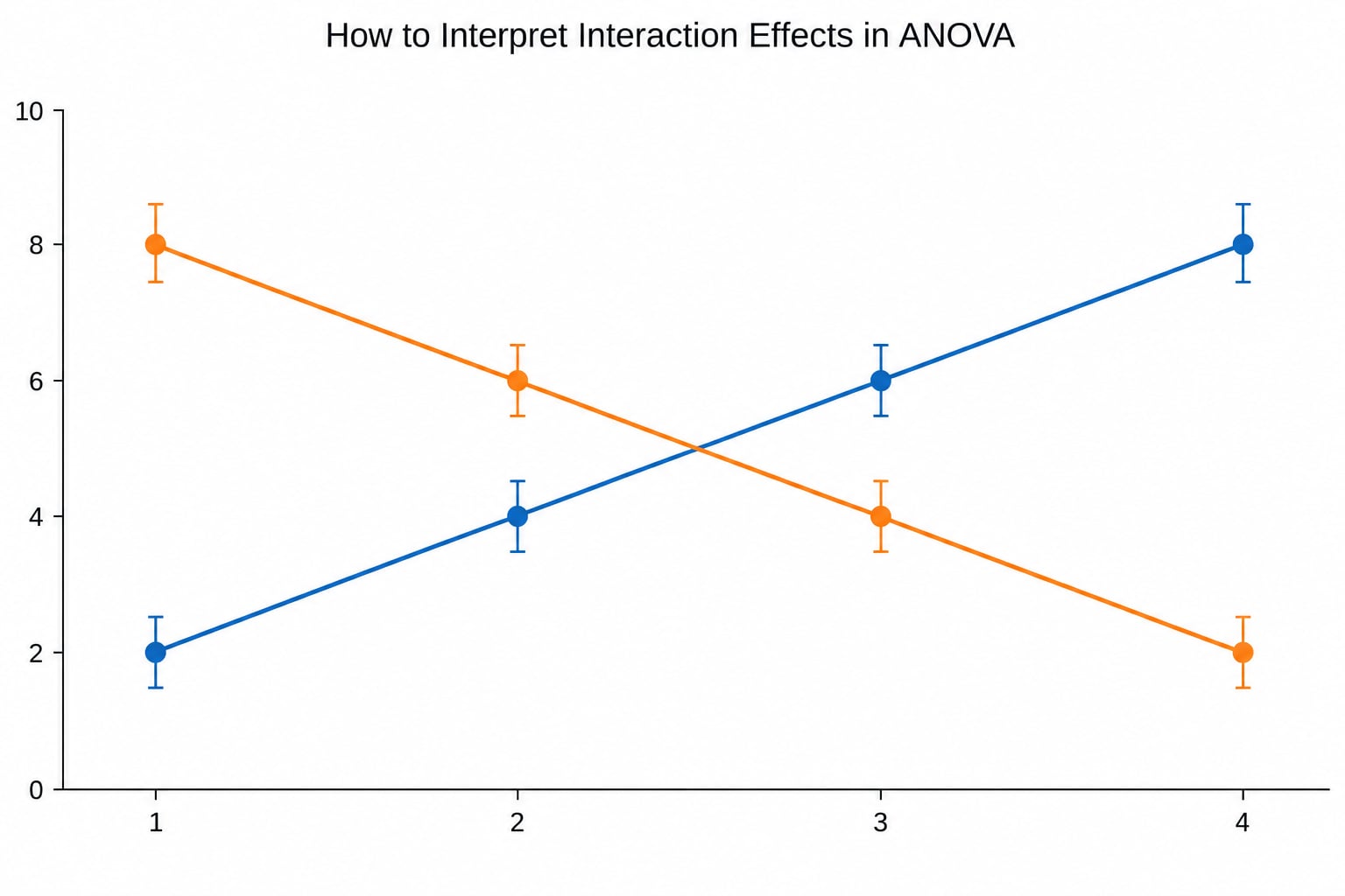
An interaction is a moderation pattern. Factor A has an effect on the outcome, and the size or direction of that effect changes at different levels of Factor B. If the lines in a plot stay flat relative to each other, there is no interaction. If they converge, diverge or cross, there is one.

Every row in an ANOVA table tests a different question. The main effect row for Factor A asks whether the marginal average across all levels of B differs between the levels of A. The A×B row asks whether those marginal averages conceal a pattern that changes with B. Both are computed from the same data, and the interaction row is the one that decides how much of the main effect story you are allowed to tell.

Because of that, the hierarchical principle applies: test the interaction first, and only interpret main effects if the interaction is not significant. A significant interaction is a gate. Once you pass through it, the main effect of A is an average across B, and averages across opposite patterns are exactly the kind of number that misleads.

The interaction row reports its own degrees of freedom, F-statistic, and p-value. For a 2×2 design the interaction has 1 degree of freedom, which is why the F value is directly interpretable as a test of whether the difference between two groups is itself different between two conditions.

What Does a Significant Interaction in ANOVA Mean?

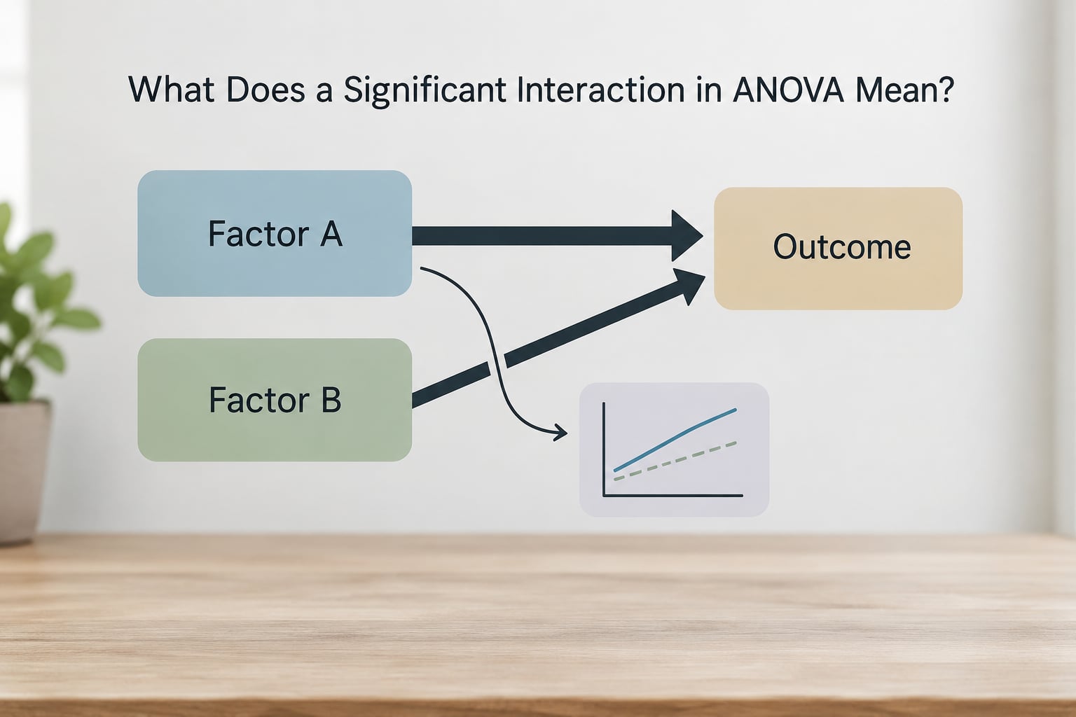
A significant interaction means the effect of one independent variable is not the same across all levels of the other. In plain terms, the difference between your groups depends on the condition they were in. Nothing about the interaction says which direction it points, and it can take three forms: ordinal, disordinal, or a mixture of the two.

An ordinal interaction happens when the lines are not parallel but never cross. One factor still pushes the outcome in the same direction at every level of the other, just with a different magnitude. A disordinal interaction, sometimes called a crossover, is where the lines cross, meaning the direction of the effect reverses between levels.

The reversal matters practically. If Method A beats Method B at low prior knowledge and loses at high prior knowledge, there is no single recommendation to give. You have a conditional finding, and the write-up has to say under which condition each method wins.

A p-value below .05 on the interaction row tells you the pattern is unlikely under a model where the factors act additively. It does not tell you the size of the effect, which is why effect size and confidence intervals belong in the same paragraph as the F and p.

Main Effects Versus Interaction Effects

Main effects are marginal means. They average each factor across all levels of the other, which is why they can be flat while the underlying pattern is dramatic. Here is how the four significance combinations change your interpretation.

Interaction	Main effects	What you report
Not significant	Both significant	Both main effects, stated as marginal averages
Not significant	One or both not significant	Report what reached significance; say the rest showed no reliable difference
Significant	Both significant	Interaction plus simple effects. Main effects are optional context, labelled as averaged across levels
Significant	None significant	Interaction plus simple effects. This is normal and not a contradiction

The third row is where most published errors happen. Reporting two significant main effects alongside a crossover interaction and stopping there means your conclusion contradicts your own table. The averaged statement can be true and still tell the reader nothing actionable.

Think of a crossover: Group A starts 8 points above Group B, and Group B ends 12 points above Group A. The marginal means land somewhere in the middle and look like a small, uninteresting gap. The interaction is the finding.

How to Read an Interaction Plot

Read the plot in a fixed order: axes first, then the vertical distance between lines at each level of the x-axis, then the error bars. The x-axis holds one factor, the y-axis holds the outcome, and each line is a level of the other factor. Lines that never touch are the visual claim of additivity.

Pattern in the plot	What it indicates	How to follow up
Parallel lines	No interaction, or one too small to detect	Interpret main effects
Converging lines	Ordinal interaction. One factor’s effect shrinks as the other increases	Simple effects for the factor whose effect shrinks
Diverging lines	Ordinal interaction in the opposite direction	Simple effects for both levels of the other factor
Crossing lines	Disordinal interaction. The effect reverses	Simple effects within each level, then report the reversal
Near-parallel but not quite	Either a small interaction or a noisy design	Rely on F, p, and confidence intervals rather than your eyes

Error bars matter more than people give them credit for. If the confidence intervals at one level of the x-axis overlap heavily while the lines look clearly separated, you may be chasing sampling noise. And a plot is not a test: eyeballing a crossover is not evidence, the F value is.

Estimated marginal means plots are the right default in SPSS and R, because they are fitted values adjusted for the design rather than raw cell averages. For unbalanced data those two can differ enough to change which line sits on top.

How to Follow Up a Significant Interaction

Once the interaction is significant, you decompose it. Simple effects tests ask which levels of Factor A differ at one specific level of Factor B, and they are the right tool when you want to describe the pattern. Simple contrasts test a narrower question, such as whether the difference between two conditions is itself different from zero, and they suit confirmatory hypotheses you specified in advance.

Plan the comparisons before you run them, because every additional test is another chance at a Type I error. A full set of comparisons across a 2×4 design is 8 tests, and at a .05 threshold the chance of at least one false positive is about a third. Bonferroni, Tukey, or Holm adjustment brings that back to a defensible level. The right choice depends on whether you planned the comparisons in advance, not on which one gives smaller p-values.

SPSS syntax for simple effects

SPSS does not produce these comparisons by default, which is the single most common source of frustration on the forums. Build the model with /METHOD=DESIGN, add /EMMEANS with COMPARE, and ask for the adjustment explicitly.

UNIANOVA score BY method(1 2) preparation(1 2)
  /METHOD = DESIGN method preparation method*preparation
  /EMMEANS = TABLES(method) COMPARE(method) ADJ(BONFERRONI)
  /EMMEANS = TABLES(preparation) COMPARE(preparation) ADJ(BONFERRONI)
  /PLOT = PROFILE(method*preparation) TYPE = LINE ERRORBAR = CI
  /PRINT = DESIGN ETASQ
  /CRITERIA = ALPHA(.05).

Run the /EMMEANS lines once for each factor you want to decompose. Reading the output: the Pairwise Comparisons table gives you the difference, the confidence interval, and the adjusted significance for each cell comparison.

R with the emmeans package

library(emmeans)
fit <- aov(score ~ method * preparation, data = d)

anova(fit)                      # the interaction row
emmeans(fit, ~ method | preparation, adjust = "holm")
emmeans(fit, ~ preparation | method, adjust = "holm")
emmip(fit, ~ preparation | method)   # interaction plot

The | operator is the whole idea in one character: everything to its left is compared within each level of the factor to its right. Swap the sides and you get the other set of simple effects.

A Step-by-Step Example of Interpreting an ANOVA Interaction

Suppose you ran a study of exam scores for 80 students. Factor A is instruction method, lecture or online. Factor B is prior preparation, low or high, with 20 students in each cell. Here is a hypothetical ANOVA table from those means, with a within-cell standard deviation of 7.

Source	SS	df	MS	F	p	Partial eta squared
Method	45	1	45.0	0.92	.34	0.012
Preparation	4,805	1	4,805.0	98.06	< .001	0.563
Method × Preparation	245	1	245.0	5.00	.028	0.062
Error	3,724	76	49.0
Total	8,819	79

The cell means behind it: lecture with low preparation 68, lecture with high preparation 80, online with low preparation 66, online with high preparation 85.

Step 1: the interaction. F(1, 76) = 5.00, p = .028. Significant at .05, so the main effects are gated. Partial eta squared of 0.062 sits right at the medium benchmark, which tells you the effect is worth writing about even though it is not dramatic.

Step 2: the direction. Under low preparation the lecture group is 2 points ahead. Under high preparation the online group is 5 points ahead. The lines cross, so this is a disordinal interaction.

Step 3: simple effects. Comparing preparation within each method, the standard error of each difference is 2.21. Lecture: 80 against 68, t(76) = 5.42, p < .001. Online: 85 against 66, t(76) = 8.58, p < .001. Preparation clearly matters, and it matters more for the online group.

Step 4: the reverse comparisons. Comparing method within each preparation level, low preparation gives t(76) = 0.90, p = .37, no difference. High preparation gives t(76) = 2.26, p = .026, which does not survive a Bonferroni correction across four planned comparisons. The honest summary is that the methods were indistinguishable at low preparation, and the difference at high preparation is suggestive rather than established.

Step 5: the main effect that vanished. Method alone, F(1, 76) = 0.92, p = .34. Averaged across preparation, lecture scores 74 and online scores 75.5, a 1.5 point gap that the design cannot support. There is no contradiction here. Two unequal gains in opposite directions average to almost nothing.

Step 6: the conclusion. Prior preparation affected exam scores overall, and its effect depended on instruction method. Well-prepared students scored higher than under-prepared students in both formats, with a larger gain online, while the two formats performed similarly among under-prepared students. The crossover means no single format is better across the board.

How to Report Interaction Effects in Your Results

Report the F, the degrees of freedom, the p-value, the effect size, and the direction, in that order. Then state which specific groups differ. Fill in the blanks and you are close to APA style.

Situation	Template
Significant interaction	There was a significant interaction between [A] and [B], F(df1, df2) = [F], p = [p], partial eta squared = [ηp²]. Simple effects showed that [specific comparison] differed at [level], t(df) = [t], p = [p], while [other comparison] did not.
Non-significant interaction	The interaction between [A] and [B] was not significant, F(df1, df2) = [F], p = [p], partial eta squared = [ηp²], so main effects were interpreted.
Three-way interaction	There was a three-way interaction between [A], [B], and [C], F(df1, df2) = [F], p = [p], partial eta squared = [ηp²], indicating that the [A] × [B] interaction varied across levels of [C].
Effect size only	Follow the p-value with partial eta squared. Rough guides: 0.01 small, 0.06 medium, 0.14 large.

Partial eta squared is easy to compute by hand: divide the effect’s sum of squares by that sum of squares plus the error sum of squares. For the interaction above, 245 divided by 245 plus 3,724 gives 0.062.

One more reporting habit worth building: report confidence intervals for the simple effects, not just p-values. A difference of 5 points with an interval running from 0.2 to 9.8 tells a reader far more than a bare p-value, and reviewers increasingly ask for it.

Common Interpretation Mistakes

Reporting main effects after a significant interaction. This is the big one. The marginal average has no clean referent, and thesis committees flag it. Report the simple effects instead, and if you mention the main effect at all, label it as averaged across levels.

Believing non-significant main effects contradict a significant interaction. They cannot. Averaging across an opposing pattern shrinks any main effect toward zero. If Method looks null and the interaction is real, the simple effects are the story.

Describing cell means instead of the pattern. Listing four numbers tells the reader nothing about direction or magnitude. Say what changes, and by how much, as the other factor moves.

Treating p > .05 as proof of no effect. A non-significant interaction means the data did not detect one at your sample size. With 20 per cell, a real but modest interaction can easily go unnoticed. Report the confidence interval around the effect size and let readers judge.

Running every possible pairwise comparison. Testing all cell differences after a significant interaction inflates your error rate and produces comparisons you have no story for. Choose the comparisons your design implies, then correct for multiplicity.

Trusting the plot over the test. Lines that look parallel may not be, and lines that cross slightly may fall short of significance. The F and p decide; the picture is for the reader.

Ignoring balance. With unequal cell sizes, raw cell means and estimated marginal means can order differently, and Type III sums of squares change the main effect tests. Check the cell counts before you interpret the main effect rows.

Frequently Asked Questions

Conclusion: Start With the Pattern, Not the p-Value

Run the interaction row first, because it decides whether your main effects are allowed to speak. If it is not significant, interpret the main effects as marginal averages and move on. If it is significant, plot it, name the pattern as convergent, divergent or crossover, run the simple effects that the design implies with a multiplicity correction, and add partial eta squared to the report.

One last practical check before you write: does the sentence describing your result make sense to someone who has not seen the table? If it only works when you mentally picture the plot, the sentence needs work. Interaction findings are conditional by definition, so the conditions belong in the sentence, not in a footnote. Software defaults and journal style requirements do shift, so confirm the current conventions for your field in 2026 before you submit.