How to Calculate Effect Size for a t Test: Simple Guide 2026

The standard effect size for a t-test is Cohen’s d, the standardized difference between two means: you divide the difference between your group means by a pooled standard deviation, and the result comes back in standard-deviation units instead of your original measurement units. If your design has matched pairs, the denominator changes to the standard deviation of the difference scores rather than a pooled value.

Knowing how to calculate effect size for a t test takes about five minutes once you have the summary numbers. The whole job is three arithmetic steps: work out the right denominator, divide the mean difference by it, then check the number against the small/medium/large benchmarks. I will walk through all four t-test variants, including Welch’s, and show every intermediate value so you can check the arithmetic yourself.

A p-value answers “could this be chance?” and nothing else. It moves when you change the sample size, which is why a study with p < .001 and 5,000 participants can have an effect size of d = 0.15, which is practically nothing. Cohen’s d keeps the answer in units people can reason about.

Table of Contents

1. 1What You Need
2. 2Step-by-Step
3. 3Independent Samples: Calculate Cohen’s d With the Pooled Standard Deviation
4. 4When to Use Hedges’ g Instead of Cohen’s d
5. 5Paired Samples: Standardize the Difference Scores, Not the Raw Scores
6. 6How to Interpret and Report the Effect Size
7. 7Common Mistakes and How to Fix Them
8. 8Frequently Asked Questions
9. 9What is a good effect size for a t test?
10. 10Should I report Cohen’s d or Hedges’ g?
11. 11Can I calculate an effect size from a t statistic?
12. 12Which effect size should I use for a paired-samples t test?
13. 13How do I calculate effect size in SPSS, JASP, Excel or R?
14. 14Is a significant t test the same as a large effect?

What You Need

Collect these before you start. If you have raw data the software does the rest, but doing one by hand teaches you which number is correct.

• Group or condition means (M1, M2). For a one-sample test, just the sample mean.
• Standard deviations (s1, s2). For a paired test, the standard deviation of the difference scores.
• Sample sizes (n1, n2). Needed for the pooled variance and for the small-sample correction.
• The t statistic and its degrees of freedom, plus the p-value, so you can report them next to the effect size.
• Whether the test is one-tailed or two-tailed, and whether you assumed equal variances.

The formula depends on the design, and that is where most mistakes happen. Pairing is a property of your data, not an option you toggle on to make a number look better.

t-test variant	Effect size formula	Software setting
One-sample	d = (m − μ) / s	rstatix: cohens_d(x, mu = 100)
Independent, Student’s (equal variances)	d = (M1 − M2) / Sp	SPSS: tick Effect size; R: cohens_d(y ~ group, var.equal = TRUE)
Independent, Welch’s (unequal variances)	d = (M1 − M2) / sqrt((s1² + s2²)/2)	R: cohens_d(y ~ group, var.equal = FALSE)
Paired	dz = mean difference / SD of difference scores	SPSS: Paired-Samples T Test > Effect size; R: cohens_d(pre, post, paired = TRUE)

Two more symbols you will meet: Sp is the pooled standard deviation, a single estimate of the population SD that assumes the two groups share one variance. df is the degrees of freedom, n1 + n2 − 2 for Student’s test and n − 1 for a paired or one-sample test.

Step-by-Step

Independent Samples: Calculate Cohen’s d With the Pooled Standard Deviation

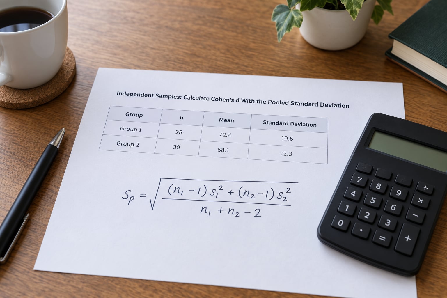
Cohen’s d for two independent groups is the difference between their means divided by the pooled standard deviation:

d = (M1 − M2) / Sp

Sp = sqrt( [ (n1 − 1)s1² + (n2 − 1)s2² ] / (n1 + n2 − 2) )

Both parts matter. Students routinely divide the mean difference by the standard deviation of just one group, which quietly assumes the two groups are equally variable.

Here is a complete example. A researcher compares reaction times for two independent groups: 24 participants in condition A and 26 in condition B.

• n1 = 24, M1 = 78.4 ms, s1 = 9.6 ms
• n2 = 26, M2 = 71.2 ms, s2 = 10.4 ms

Step 1, square the standard deviations: 9.6² = 92.16 and 10.4² = 108.16.

Step 2, multiply each by its degrees of freedom: 23 × 92.16 = 2119.68 and 25 × 108.16 = 2704.00.

Step 3, add and divide by the total df of 48: (2119.68 + 2704.00) / 48 = 4823.68 / 48 = 100.49.

Step 4, take the square root: Sp = sqrt(100.49) = 10.02.

Step 5, divide the mean difference by it: d = (78.4 − 71.2) / 10.02 = 7.2 / 10.02 = 0.72.

That is a large effect in Cohen’s terms. Check it against your t output: the standard error of the difference is Sp × sqrt(1/n1 + 1/n2) = 10.02 × 0.283 = 2.84, so t = 7.2 / 2.84 = 2.54 with df = 48, and p is under .02. The effect size and the test agree, which is how you know the arithmetic holds.

When you cannot compute Sp at all, the t statistic and degrees of freedom are enough. For the independent case, d = t × sqrt(1/n1 + 1/n2). With equally sized groups that simplifies to d = 2t / sqrt(df), so a reported t(24) = 3.00 gives d = 6.00 / 4.90 = 1.22. Useful when you are working from a paper that reported the test statistic and nothing else.

Welch’s test does not assume equal variances, so it uses the root-mean-square of the two standard deviations instead of the pooled estimate: sqrt((s1² + s2²) / 2). With equal group sizes and equal variances it returns the same number as Cohen’s d. When group sizes differ, a Monte Carlo comparison of estimators for the Welch case found Cohen’s d_A less biased than the alternatives while Hedges’ g matches the pooled version, so d_A is the safer choice to quote. Glass’s delta is another option: divide by the control group’s standard deviation alone, useful when one group is a genuine baseline.

The worked example above uses equal-ish group sizes where the two denominators barely differ. When variances are far apart, say s1 = 9.6 and s2 = 20.0, the pooled version shrinks the denominator and inflates d. That is not an error, it is the assumption doing its job, but it is worth naming in your write-up.

When to Use Hedges’ g Instead of Cohen’s d

Cohen’s d is biased upward in small samples, and the bias is not subtle: below about 20 participants per group it can inflate the estimate by a noticeable margin. Hedges’ g fixes that with a correction factor J that shrinks d slightly:

J = 1 − 3 / (4(n1 + n2) − 9)

g = J × d

Apply it to the example. With a total N of 50, J = 1 − 3 / (4 × 50 − 9) = 1 − 3/191 = 0.9843, so g = 0.9843 × 0.72 = 0.71. Barely different, because N = 50 is not small.

Try it at N = 20 instead: J = 1 − 3 / (80 − 9) = 1 − 3/71 = 0.9577. A d of 0.72 becomes g = 0.69. The correction grows as N shrinks, which is exactly the point.

Report one or the other, not both, and name it. “The two groups differed by a large amount, d = 0.72” and “Hedges’ g = 0.69” answer different questions about the same data, and a reader who sees both will wonder which one you meant. If your sample is small, say why you used g. Most styles guide allows either measure as long as the choice is stated.

Paired Samples: Standardize the Difference Scores, Not the Raw Scores

For a paired or dependent t-test, you do not use the pooled standard deviation. You compute one difference score per participant, then divide the mean of those differences by their own standard deviation:

d_z = mean(D) / s_D

where D is the set of difference scores and s_D is their standard deviation.

Worked example. Thirty students take a pre-test and a post-test: pre M = 54.2 with SD = 8.1, post M = 60.8 with SD = 7.6. The mean gain is 6.6 points and the standard deviation of the 30 difference scores is 4.9, so d_z = 6.6 / 4.9 = 1.35.

Compare that with the number you get by dividing the gain by the pooled SD of the two test occasions, sqrt((29 × 65.61 + 29 × 57.76) / 58) = 7.85, giving 6.6 / 7.85 = 0.84. The paired version is the correct one, and the reason is simple: the difference scores carry the variation that matters, while the raw scores carry each student’s stable starting level.

This is the confusion that shows up again and again in forums, where people ask whether paired-sample d uses the same formula as the independent case. It does not, and the difference can be large whenever pre-test and post-test scores are strongly correlated.

Check it against t again. With n = 30, the standard error of the mean difference is 4.9 / sqrt(30) = 0.895, so t = 6.6 / 0.895 = 7.38 with df = 29. The shortcut is d_z = t / sqrt(n): 7.38 / 5.48 = 1.35. The same relationship in reverse, and it works because d_z standardizes by n rather than by n − 1.

Two labels circulate for this value. Cohen’s original d for repeated measures was the mean difference divided by the post-test or pooled SD, which is smaller and reads as more conservative. Most modern software reports d_z as shown above, and meta-analyses that mix d and d_z end up with biased pooled estimates. Check which convention each study used before combining them.

How to Interpret and Report the Effect Size

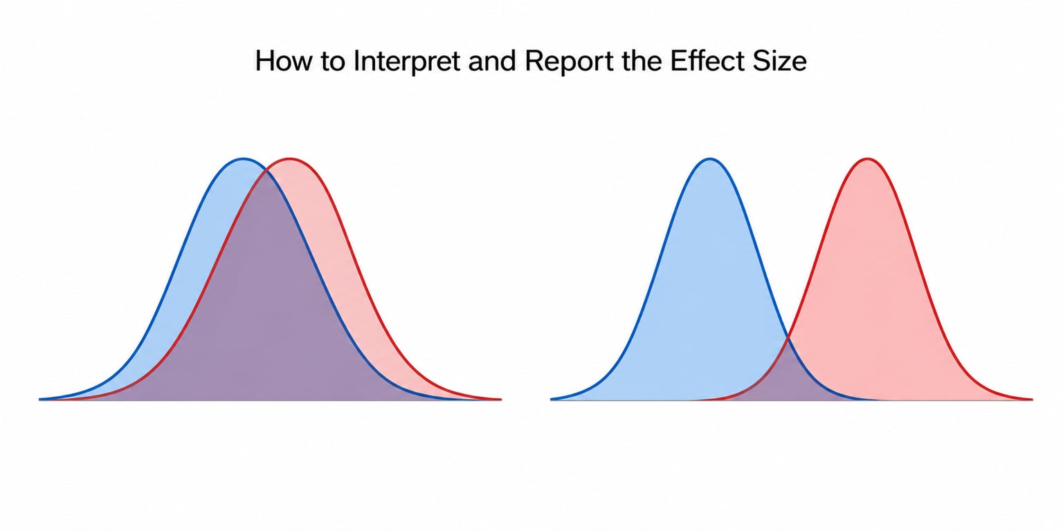
Cohen’s benchmarks of 0.2, 0.5 and 0.8 for small, medium and large are the ones to quote, but treat them as field-relative rather than universal. A d of 0.2 on a reaction-time measure is trivial; the same d on a quality-of-life scale can matter a great deal.

Cohen’s d	Label	Point-biserial r	Distribution overlap	Sample size per group for 80% power at α = .05
0.2	Small	0.10	About 61%	394
0.5	Medium	0.24	About 38%	64
0.8	Large	0.37	About 15%	26

The point-biserial column is the correlation between the outcome and the group label, which is the effect size family used in ANOVA and regression. The conversion is exact for independent designs: r_pb = d / sqrt(d² + 4), and the equivalent r = sqrt(t² / (t² + df)). Use it when you are trying to compare a t-test result with an F-test or with R² reported elsewhere.

For a one-way ANOVA run on the same two groups, partial eta squared works out to t² / (t² + df). With t = 2.54 and df = 48, that is 6.45 / 54.45 = 0.118. Same result, different scale, and it lets your t-test sit in a table next to your other outcomes.

The APA results sentence puts it all together: A reaction times were significantly slower in condition A (M = 78.4, SD = 9.6) than in condition B (M = 71.2, SD = 10.4), t(48) = 2.54, p = .014, d = 0.72.

Add a confidence interval for the effect size where you can. Most software can produce one, and the intervals are wide in small samples, which is the honest picture. A point estimate of 0.72 with a 95% interval running from 0.28 to 1.15 tells a reader far more than the point estimate alone.

In SPSS, go to Analyze > Compare Means > Independent-Samples T Test, put the outcome in Test Variable(s) and the grouping variable in Group(s), click Define Groups and assign the two values, then tick Effect size under Options before pressing OK. The output adds Cohen’s d and its significance test to the group statistics table. Cohen’s d only became a built-in option in SPSS 27, so anyone on an older copy has to compute it by hand or use a spreadsheet add-in. For paired data the path is Analyze > Compare Means > Paired-Samples T Test with the same Effect size box.

JASP prints Cohen’s d alongside the group statistics in its Independent-Samples T Test panel without any extra setting, and the paired panel has an Effect size checkbox for d. In Excel, put n1, M1, s1, n2, M2, s2 in six cells and write =(B3-B6)/SQRT(((B2-1)*B4^2+(B5-1)*B7^2)/(B2+B5-2)) for d. In R, rstatix::cohens_d() handles every variant through its arguments:

library(rstatix)
cohens_d(score ~ group, data = df, var.equal = TRUE)   # Student's
cohens_d(score ~ group, data = df, var.equal = FALSE)  # Welch's
cohens_d(pre, post, paired = TRUE)                     # paired
cohens_d(x, mu = 100)                                  # one-sample

Stata’s ttest reports the mean difference and its confidence interval but not d, so compute it from the summary statistics or run regress followed by cohend. For planning, G*Power takes a target d directly and returns the sample size you need per group.

Common Mistakes and How to Fix Them

Using the independent formula on paired data. The denominator has to be the standard deviation of the difference scores. Reuse the paired procedure above and the numbers will match your software.

Standardizing by the wrong standard deviation. In an independent design, divide by the pooled SD, not by the SD of the group you happened to run first.

Skipping the small-sample correction. Below roughly 20 per group, report Hedges’ g rather than Cohen’s d and say that you did.

Deriving the effect size from the p-value. A p-value and sample size cannot tell you the size of the effect in units of the variable. You need a mean difference and a standard deviation, or at minimum a t statistic with its degrees of freedom.

Reading a negative d as an error. The sign follows the order you subtracted the groups in. If group A came second, d comes out negative. Report the absolute value as the magnitude and say which group was higher.

Getting a different d from a second tool. Three causes account for nearly all of it: pooled versus Welch denominator, Hedges’ correction on versus off, and paired versus independent handling. Change one setting at a time until the two agree, then state your choices in the write-up.

Two more cases worth knowing. If all you have is an adjusted or model-estimated mean, you usually cannot recover a valid standardized effect, because standardized measures need the raw sample SD. And if the normality or equal-variance assumption fails badly, report a non-parametric companion such as the rank-biserial correlation or Cliff’s delta alongside the t-test rather than defending the parametric result.

Frequently Asked Questions

Start with your design. If the groups are independent and roughly equally variable, compute the pooled standard deviation and divide the mean difference by it. If the scores are paired, work from the difference scores. Either way, add a confidence interval where your software offers one, report the t statistic, degrees of freedom, p-value and effect size in the same sentence, and then say whether the size of the difference matters in your field. That last part is the only judgement a formula cannot make for you.