How to Run a t Test in R: A Simple Guide for 2026

To run a t test in R, use the built-in t.test() function. Pass your numbers as t.test(x) for a one-sample test, t.test(y ~ group, data = df) for two independent groups, or add paired = TRUE for matched measurements. Nothing needs installing, because t.test() lives in base R.

The syntax is the easy part. Nearly every wrong result I have seen comes from picking the wrong variant for the data shape, so the real work happens before you type anything: decide whether your observations are linked, write down the reference value your hypothesis compares against, and check the assumptions the test needs.

This guide walks through that sequence with runnable code and full console output you can copy straight into RStudio.

Table of Contents

1. 1What You Need Before You Start
2. 2Step-by-Step: How to Run a t Test in R
3. 3Step 1: Load and Inspect Your Data
4. 4Step 2: Choose the Right t Test for Your Data
5. 5Step 3: Check Assumptions and Pick the R Method
6. 6Step 4: Run the t Test in R and Read the Console Output
7. 7Step 5: Interpret the R Output
8. 8Step 6: Report the Result in APA Style
9. 9Common Mistakes That Quietly Break the Analysis
10. 10Frequently Asked Questions
11. 11How do I perform a t test in RStudio?
12. 12How do I run a 2 sample t test in R?
13. 13Should I use the Welch or the Student t test in R?
14. 14How do I check if my data is normal before a t test?
15. 15What do I do when my t test and Wilcoxon test disagree?
16. 16How do I report a t test result in APA format?
17. 17Conclusion

What You Need Before You Start

You need four things, and only one of them is software.

1. R and, ideally, RStudio. R is the language. RStudio is the free desktop front end that adds a data viewer, a script pane and a console side by side, which makes the steps below far easier to follow. If you already have R, everything here works in the plain console too.

2. A numeric outcome variable. That is the thing you are comparing: a score, a reaction time, a length, a balance measurement. If your outcome is a count of successes, a rating on a five-point scale, or a percentage bounded at zero and one, stop, because a t test is the wrong tool.

3. A written hypothesis with a reference value. For a one-sample test this is the number you are comparing against, passed as mu =. For a two-sample test it is the assumption that both group means are equal, which is built in and never written down.

4. A decision about pairing. Ask whether the two sets of numbers are matched to each other. Scores from the same people before and after a training programme, measurements from the left and right eye of the same participant, twins, repeated readings from the same instrument, those are all paired. Different people in a treatment arm and a control arm are independent. This one question decides which function call you need, and it comes from your study design, not from the data.

One more practical note: get the data into the right shape. A two-sample test wants one numeric column plus a group column with two levels. A paired test wants one row per participant with the two measurements in two columns. If your before and after values are stacked in a single column with a label beside them, you will need to reshape them, which I show in Step 4.

Step-by-Step: How to Run a t Test in R

Step 1: Load and Inspect Your Data

Start by looking at the data before testing it, because almost every confusing error later on is really a data shape problem hiding in plain sight.

For a real project, read your file in and check it. This is the whole routine:

library(readr)
df <- read_csv("study_data.csv")

str(df)                      # structure: column types, row count
head(df)                     # first six rows
summary(df$outcome)          # mean, quartiles, missing count
table(df$group, useNA = "ifany")   # how many in each group

Read the output of table() carefully. If it prints NA for a group, you have rows with a missing label, and those rows cannot be assigned to either group.

For the examples in this guide I will use vectors defined in the script itself, so you can run every line from here without a data file:

scores <- c(78, 84, 90, 86, 92, 88, 76, 95)

What to look for: one numeric outcome column, a group column with exactly two levels, no stray text in the numeric column, and a row count that matches your expectation.

Step 2: Choose the Right t Test for Your Data

Answer two questions in order. How many groups do you have, and are the two sets of numbers linked to the same participants?

Question one: one group or two? If you have a single set of measurements and want to compare its mean to a known number, you need a one-sample t test. If you have two sets, you need a two-sample test.

Question two: linked or not? If each number in set A belongs to the same unit as a specific number in set B, you need a paired test. If the two sets are separate people or separate units, you need an independent two-sample test.

Variant	Data shape	Null hypothesis	Typical use
One-sample	One numeric vector	Sample mean equals mu	A sample mean versus a specification or published value
Welch two-sample	Two independent groups	Both group means are equal	The default for independent groups, such as treatment versus control
Student two-sample	Two independent groups with similar variances	Both group means are equal	Only when you have a good reason to assume equal variances
Paired	One row per matched unit, two columns	Mean difference equals zero	Before and after measurements, matched pairs, repeated readings

Worth knowing: R gives you Welch by default for two independent samples, and that default is the right one most of the time. It does not assume equal variances and it stays correct when group sizes differ. You only switch to Student with var.equal = TRUE when you have a real reason, not because an old tutorial told you to.

Step 3: Check Assumptions and Pick the R Method

A t test makes three assumptions, and the first one is not really a testable statistic. It is about design.

Independence. Each observation should be independent of the others. Participants measured repeatedly, classrooms nested in schools, or villages in the same district all break this assumption, and no amount of checking in R will rescue it.

Approximate normality of the data, or a large enough sample. The t test is sensitive to badly skewed data when samples are small. The central limit theorem is your friend once each group has roughly 30 or more observations; below that, look at the shape.

shapiro.test(scores)

hist(scores)
qqnorm(scores); qqline(scores)

The shapiro.test() output gives you a W statistic and a p-value. Read it the standard way: a p-value above 0.05 means you do not reject normality, and a p-value below 0.05 means the data depart from a normal shape enough to matter at your sample size. Always look at the histogram and the Q-Q plot as well. A straight line with points hugging it supports the assumption; a curve or a tail of points drifting away does not. With only eight observations the Shapiro test has very little power, so judge the shape of the data rather than the p-value alone.

Equal variances, for the Student test only. Welch does not need this. If you are considering var.equal = TRUE, test the assumption first:

a <- c(12, 15, 14, 13, 16, 15, 14, 13, 12, 14)
b <- c(10, 11, 13, 12, 12, 11, 10, 13, 11, 12)

var.test(a, b)

The output is an F statistic with degrees of freedom and a p-value. Here F is 1.4857 with 9 and 9 degrees of freedom, a p-value well above 0.05, so the two variances are not detectably different. That result would permit a Student test, though Welch remains the safer default.

One more assumption check that people often skip: outliers. A single wildly wrong value inflates the variance of its group and can make a real difference disappear. Check with boxplot(), and decide whether the value is a data error or a legitimate extreme observation before you delete anything.

Step 4: Run the t Test in R and Read the Console Output

Here is the same hypothesis run four ways, with the full console output each time.

One-sample t test. The null says the population mean is 88. The mu argument supplies that reference value.

t.test(scores, mu = 88)

#  One Sample t-test
#
# data:  scores
# t = -0.80386, df = 7, p-value = 0.4472
# alternative hypothesis: true mean is not equal to 88
# 95 percent confidence interval:
#  80.6089 91.6411
# sample estimates:
# mean of x
#  86.125

If your data are in a data frame column, use the same function with column names rather than vectors: t.test(df$outcome, mu = 88).

Two independent groups, Welch version. Using the vectors from Step 3:

t.test(a, b)

#  Welch Two Sample t-test
#
# data:  a and b
# t = 4.2709, df = 17.338, p-value = 0.0004931
# alternative hypothesis: true difference in means is not equal to 0
# 95 percent confidence interval:
#  1.1648 3.4352
# sample estimates:
# mean of x
#  13.8
#
# mean of y
#  11.5

Two independent groups, Student version. The only change is the variance argument, and the degrees of freedom drop from 17.338 to 18 because the pooled variance estimate uses both groups symmetrically:

t.test(a, b, var.equal = TRUE)

#  Two Sample t-test
#
# data:  a and b
# t = 4.2709, df = 18, p-value = 0.0004615
# alternative hypothesis: true difference in means is not equal to 0
# 95 percent confidence interval:
#  1.1648 3.4352
# sample estimates:
# mean of x
#  13.8
#
# mean of y
#  11.5

With ten observations per group the interval is identical, which is expected: equal group sizes make the pooled and Welch standard errors the same number. Unbalance the group sizes and the two versions start to disagree, which is exactly when Welch earns its keep.

The formula interface with a built-in dataset. For a data frame, the two-sample form takes a formula:

t.test(len ~ supp, data = ToothGrowth)

#  Welch Two Sample t-test
#
# data:  len and supp
# t = 1.9153, df = 55.309, p-value = 0.06063
# alternative hypothesis: true difference in means between len and supp is not equal to 0
# 95 percent confidence interval:
#  -0.1710732 7.5714032
# sample estimates:
# mean of x
#  18.813
#
# mean of y
#  19.733

Note the group column. R treats the right-hand side as a factor automatically, which is why the formula form rarely complains. The vector form is fussier, and if your group column is numeric rather than a factor you will get a confusing error rather than a test. Convert it first:

df$group <- factor(df$group)
t.test(outcome ~ group, data = df)

Paired t test. The two vectors must be in the same order, row for row, because R matches them by position and never checks that you meant to.

before <- c(120, 132, 118, 145, 129, 137, 155, 128)
after  <- c(132, 141, 125, 152, 138, 145, 160, 136)

t.test(after, before, paired = TRUE)

#  Paired t-test
#
# data:  after and before
# t = 11.314, df = 7, p-value = 3.501e-05
# alternative hypothesis: true mean difference is not equal to 0
# 95 percent confidence interval:
#  6.4269 9.8231
# sample estimates:
# mean difference
#  8.125

Notice what the output does not print: the two group means. It prints the mean difference, 8.125, because the paired test runs on the within-participant differences.

Run the same before and after data as if the two sets were unrelated and the picture changes completely:

t.test(after, before)

#  Welch Two Sample t-test
#
# data:  after and before
# t = -2.7294, df = 11.585, p-value = 0.01933

t drops from 11.3 to 2.7 and p climbs from 0.000035 to 0.019. The data did not change, only the assumption did. Discarding the pairing throws away the strong correlation within each person and makes a clear effect look marginal. This is the single most common way people get a weaker result than their study deserves.

One-sided tests. Set the direction with alternative, and be honest about the timing:

t.test(len ~ supp, data = ToothGrowth, alternative = "less")

#  Welch Two Sample t-test
#
# data:  len by supp
# t = 1.9153, df = 55.309, p-value = 0.03032

"less" tests whether the mean of x is smaller than the mean of y, "greater" tests the reverse, and "two.sided" is the default. Choose the direction from your hypothesis and write it down before you look at the results, because a one-sided test halves your p-value by design, and choosing the direction after seeing the data is a form of cheating that reviewers notice.

Reshaping long data for a paired test. This is where beginners lose an afternoon. Suppose your before and after scores sit stacked in one column with a time label beside them, one column per participant per time point:

library(tidyr)
wide <- long_df %>% pivot_wider(names_from = time, values_from = score)
t.test(wide$after, wide$before, paired = TRUE)

The two columns after and before now come out of the pivot in matching row order, which is what the paired test needs.

A bootstrap confidence interval. When the normality assumption worries you, ask for the interval directly instead of trusting the t-based one:

set.seed(42)
boot_diff <- replicate(10000,
  mean(sample(a, length(a), replace = TRUE)) -
  mean(sample(b, length(b), replace = TRUE)))
quantile(boot_diff, c(0.025, 0.975))

If the bootstrapped interval is close to the one t.test() printed, the t-based interval is trustworthy. If it is much wider or shifted, your sample is too small for the assumption to hold and you should say so.

Step 5: Interpret the R Output

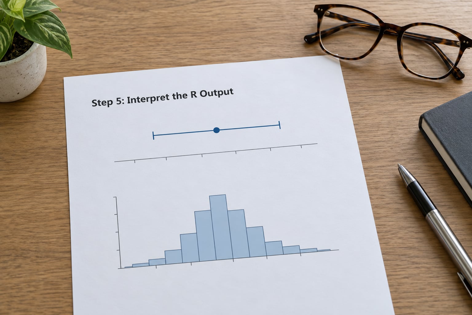
Every t.test() result contains the same six fields. Here is what each one means, using the one-sample result from Step 4.

t statistic. The observed difference between the sample mean and the null value, divided by the standard error of that difference. It is a standardised distance, which is why it can be compared across studies. A t of -0.804 means the sample mean sits slightly below 88, in units of standard error. The sign tells you the direction; the size tells you the distance.

Degrees of freedom. How much information the estimate has behind it, 7 here because eight observations lost one degree estimating the mean. Smaller samples give smaller df and a heavier t distribution, so the same t is less convincing. Welch reports fractional df, such as 17.338, because it uses the Welch-Satterthwaite correction rather than assuming equal variances.

p-value. The probability of seeing a t at least this extreme if the null hypothesis were true. At p = 0.4472 in that one-sample run, the data are completely consistent with a true mean of 88, so you do not reject the null. Small p values mean the observed gap is hard to explain by sampling noise. Note the wording: you never accept the null, you simply fail to reject it. Absence of evidence is not evidence of absence.

Confidence interval. Here, 80.61 to 91.64. If you ran this sampling exercise many times, intervals built this way would capture the true mean about 95 percent of the time. In this run the interval contains 88, which is the same conclusion as the p-value, said more usefully. Report the interval alongside the p-value whenever you can, because readers care far more about the size of the effect than about whether it squeaked past 0.05.

Sample estimates. The group means themselves, 86.125 in the one-sample case and 13.8 against 11.5 in the two-group case. These are the numbers that tell the actual story. A difference can be statistically detectable and still be trivially small in practice.

Mean difference, for paired tests only. 8.125 units, with an interval of 6.43 to 9.82. The paired output replaces the two means with this single quantity.

One thing the output does not contain is effect size, and this is where many reports stop too early. For a one-sample or paired test, Cohen’s d is a division:

# one-sample or paired: d = t / sqrt(n)
d_one  <- 0.80386 / sqrt(length(scores))   # 0.284
d_pair <- 11.314  / sqrt(length(before))   # 4.000

# two independent groups: use the pooled standard deviation
pooled_sd <- sqrt(((length(a) - 1) * var(a) + (length(b) - 1) * var(b)) /
                   (length(a) + length(b) - 2))
d_two <- (mean(a) - mean(b)) / pooled_sd    # 1.91

The rough reading is 0.2 small, 0.5 medium, 0.8 large, with 1.2 very large. The paired example scores 4.00, a difference so large that the label stops carrying information. Say the direction and the raw units in that case, for example that scores rose by 8.13 points, rather than reporting a large multiple.

The habit worth building: read the confidence interval first, the effect size second, and the p-value last. Statistical significance only answers whether a difference is detectable in this sample. The interval and the effect size answer whether anyone should care.

Step 6: Report the Result in APA Style

Reporting is where a lot of good analysis goes to waste, usually because the reader has to reverse-engineer the sentence from the console output. Here is the mapping, so you can write it directly.

Output field	What to write	Example
t statistic	The letter t and the value, two or three decimals	t = 4.27
df	Degrees of freedom; round Student df up, keep Welch df to two decimals	df = 18
p value	p for values above .05, p < .001 for smaller ones, never p = 0	p < .001
Confidence interval	The 95 percent interval, or 90 percent for a one-sided test	95 percent CI [1.16, 3.44]
Means	Raw group means, with standard deviations or standard errors	M = 13.8 (SD = 1.32)
Effect size	Cohen’s d with its value	d = 1.91

One APA sentence per variant, using the numbers from Step 4:

A one-sample t test showed that the sample scores (M = 86.13, SD = 6.60) did not differ significantly from the reference value of 88, t(7) = -0.80, p = .447, 95 percent CI [80.61, 91.64].

An independent-samples t test showed that group A (M = 13.80, SD = 1.32) scored higher than group B (M = 11.50, SD = 1.08), t(18) = 4.27, p < .001, 95 percent CI [1.16, 3.44], d = 1.91.

A paired-samples t test showed that scores increased significantly after the programme, t(7) = 11.31, p < .001, 95 percent CI [6.43, 9.82], d = 4.00.

Three details catch people out. Write p without a leading zero and with no equals sign, because p is never exactly zero. Italicise the statistical symbols t, p, M, SD, r and d, but not the letters of the test name. And always name the test variant, because a bare t statistic with no degrees of freedom and no variant is uninterpretable.

If you are building a results table for a paper with many rows, turn the result object into a tidy data frame:

library(broom)
res <- t.test(len ~ supp, data = ToothGrowth)
broom::tidy(res)

That returns a one-row data frame with the estimate, the statistic, the p value, the parameter and the confidence limits, ready to bind_rows() with the rest of your results.

Common Mistakes That Quietly Break the Analysis

Treating paired data as independent. The cost is real: in the example above, p rose from 0.000035 to 0.019. Ask whether rows are linked before anything else.

Using an independent test on rows that are out of order. R matches paired values by position and never verifies your intent. If your data were sorted differently between the two columns, you get a plausible-looking number that is simply wrong.

Leaving the group column as a number. A numeric group column makes the formula interface fail or compare nonsense. Convert it with factor() first.

Confusing the two calling styles. t.test(a, b) takes two vectors, while t.test(y ~ group, data = df) takes a formula. Mixing them produces the error “object ‘group’ not found” or a missing-data error. Pick one style and stay with it.

Forgetting that missing values are dropped silently. t.test() uses complete cases, so rows with an NA disappear without a warning beyond the sample size in the output. Check first with sum(is.na(df$outcome)), and be explicit with na.action = na.omit or na.rm = TRUE where those arguments apply.

Choosing a one-sided test after seeing the data. This inflates significance by design. Decide the direction from the hypothesis, not from the output.

Running pairwise t tests across three or more groups. Six comparisons at the conventional threshold gives a family-wise error rate near 24 percent. Use a one-way ANOVA with Tukey adjustment instead.

Losing the raw data. If you only have a mean, a standard deviation and a sample size, you can still run the test. For two independent groups, plug them into the standard error directly: se <- sqrt(sd1^2/n1 + sd2^2/n2), then t <- (mean1 - mean2) / se. Welch degrees of freedom follow from the same four numbers. You cannot check normality, inspect outliers or compute a confidence interval from summary statistics alone, so keep the raw file when you can.

Reading the confidence interval as a range of the data. It is a range for the mean difference, not for individual observations. A 95 percent CI from 1.16 to 3.44 says nothing about where a single participant’s score falls.

Concluding that a non-significant p means the groups are the same. It means this sample could not detect a difference. With a wide interval and a plausible important effect still inside it, the honest answer is that the study is underpowered, not that the effect is zero.

Frequently Asked Questions

Conclusion

Start by naming your design. One group or two, and are the observations linked to each other or not, because that single answer decides which t.test() call you write.

Then inspect the data, check the outcome is numeric and the group column is a factor, count the missing values, and reshape paired data into one row per participant. Run the test, let Welch handle two independent groups, and read the confidence interval before the p value. Reporting the means, the estimate and its interval, and Cohen’s d tells a reader far more than a bare p value ever will.