To get started with R for research data analysis, you install two things, put your data file in a project folder, then work through a fixed sequence: load, inspect, clean, explore, test, save. Most beginners stall in the first hour because they do not know which program to open, so the path below starts there.
The whole workflow fits into an afternoon of setup and a week or two of practice. No programming background is required, and none of the seven steps need anything beyond free software. What you do need is a dataset you understand well enough to argue about, and a question it can plausibly answer.
R is a free, open-source language built for statistical computing. RStudio Desktop is the free front end most people learn on, and it is where you will actually spend your time typing. The distinction trips up almost every newcomer, so it comes first.
Table of Contents
- 1What You Need
- 2Step-by-Step
- 3Step 1: Install R and RStudio Desktop
- 4Step 2: Create a Research Project and Load Your Data
- 5Step 3: Inspect Variables and Data Quality
- 6Step 4: Clean and Prepare the Data
- 7Step 5: Explore Patterns Before Choosing an Analysis
- 8Step 6: Run Your First Research Analysis
- 9Step 7: Check Assumptions and Save the Results
- 10Common Mistakes
- 11Frequently Asked Questions
- 12How long does it take to learn R for data analysis?
- 13What is the difference between R and RStudio?
- 14Is Python or R harder to learn?
- 15Which R packages do I actually need as a beginner?
- 16How should I handle missing data in R?
- 17Conclusion
What You Need
Four things. That is the whole shopping list, and three of them you already have.
- R itself, downloaded from CRAN, the Comprehensive R Archive Network, which is the official distribution site run by a small group at a university in New Zealand.
- RStudio Desktop, the free open-source edition. This is the program with the script pane, console and data viewer.
- One data file in CSV, Excel, SPSS or Stata format. Start small: a few hundred rows beats a few hundred thousand when you are learning.
- A written research question in plain language. Something like “does weekly study time differ between students who pass and fail” is enough to start.
Also make a project folder before you install anything, and give it a plain name with no spaces or special characters. My first one was called “Thesis FINAL v2 (do not use)” and it cost me an afternoon.
One more piece of honesty about versions: R and RStudio release on their own schedules, so menu labels and window layouts shift slightly between operating systems and between releases. If your screen does not match a screenshot exactly, look for the word, not the pixel.
Step-by-Step
Seven steps, in order. Skipping ahead is how people end up running a t-test on data they never looked at.
Step 1: Install R and RStudio Desktop
Install R first, then RStudio Desktop. The order matters because RStudio connects to an R installation on your machine and will look for it on startup.
Go to CRAN, choose your operating system from the download list, and follow the installer prompts. The defaults are fine. Then download RStudio Desktop from Posit, the company that maintains it, and install that too. When RStudio opens, the bottom-right pane should show an R version number rather than an error.
Two things people miss here. First, on Windows, R sometimes installs to a path with a version number in it, and if you later upgrade R the old path can break shortcuts; re-running the installer usually repairs it. Second, you do not need R installed on a server or through a package manager to follow this guide.
Step 2: Create a Research Project and Load Your Data
Use projects. In RStudio, go to File, then New Project, then New Directory, and give it a name. RStudio creates a folder with a subfolder called data for your files.
Put your CSV in that data folder. Then create a script with Ctrl+Shift+N (Cmd+Shift+N on a Mac) and run three lines:
library(readr)
mydata <- read_csv("data/survey.csv")
head(mydata)
Excel files need the readxl package, SPSS files need haven and read_sav(), and Stata files use read_dta() from the same package. The pattern never changes: install the package once, load it, read the file into a data frame.
You have succeeded when head(mydata) prints your first six rows with column names above them. If you see an empty table or a file-not-found message, check the working directory with getwd() before anything else.
Step 3: Inspect Variables and Data Quality
Never analyse a variable you have not looked at. Four functions tell you almost everything you need.
glimpse(mydata)
summary(mydata)
names(mydata)
str(mydata)
glimpse() shows the type of each column, which is how you spot a numeric variable that came in as text because someone typed “n/a” into it. summary() gives the mean, spread and number of missing values for numbers, and counts for categories. names() lists the column labels, and str() shows the structure in a compact way.
Look for three specific problems: numbers coded as category labels, missing values sitting in a column you assumed was complete, and response codes like 1, 2, 99 that mean something completely different from what they look like. A “9” for age is frequently a refusal code, not a nine-year-old.
Step 4: Clean and Prepare the Data
Clean in a script, never by editing the spreadsheet. Your raw file stays exactly as collected, and the cleaning becomes something you can show a reviewer.
library(dplyr)
clean <- mydata |>
  select(id, age, hours_studied, pass) |>
  rename(study_hours = hours_studied) |>
  filter(!is.na(age), age < 100) |>
  mutate(pass = recode(pass, "1" = "Pass", "0" = "Fail"))
select() keeps the columns you need, rename() fixes labels, filter() drops rows, and mutate() creates or recodes. The vertical bar is the pipe, and it passes the object on the left into the next function so you can read the steps in order.
For missing data, decide on a rule before you decide on a method. If a handful of values are missing at random, complete-case analysis is defensible and easy to describe. If most of a column is missing, or missingness is itself related to your outcome, say so in your methods section rather than quietly deleting rows.
Step 5: Explore Patterns Before Choosing an Analysis
Plots and frequency tables tell you which analysis is even appropriate. Skipping this is how people run a t-test on a heavily skewed outcome and get a result their supervisor rightly distrusts.
hist(clean$age)
table(clean$pass)
clean |>
  group_by(pass) |>
  summarise(mean_hours = mean(study_hours), n = n())
You are looking for distribution shape, group sizes, obvious outliers, and whether the relationship between variables looks linear. A histogram with one long right tail suggests you need a non-parametric test. Groups of three or four people should never be compared with a t-test at all.
Step 6: Run Your First Research Analysis
Start with something you can interpret in one sentence. Comparing study hours between pass and fail groups is a good first analysis.
result <- t.test(study_hours ~ pass, data = clean)
print(result)
The formula reads left side as outcome, right side as grouping variable. In the output, the estimate is the difference in group means, the confidence interval is the plausible range for that difference, and the p-value is the probability of seeing a gap at least this large if there were no real difference in the population.
Report the estimate and the interval first, the p-value second. A p-value of 0.03 with an estimate of 0.4 hours is a result you should not build a conclusion on, however it reached significance. Statistical significance and practical importance are different questions, and reviewers know the difference.
For more than two groups, aov(y ~ group, data = clean) runs a one-way ANOVA. For a continuous predictor, lm(outcome ~ predictor, data = clean) fits a linear regression, and the same formula handles several predictors at once.
Step 7: Check Assumptions and Save the Results
Most common tests assume roughly normal residuals within groups and roughly equal spread between them. Two quick checks cover it:
boxplot(study_hours ~ pass, data = clean)
plot(lm(study_hours ~ age, data = clean))
The residual plot for a regression should look like a random scatter around zero. If it curves, you need a different form. A failed assumption is not a dead end; it tells you to transform the variable, use a robust alternative, or report what you did and why.
Now save everything. Write your cleaned data with write_csv(clean, "data/clean.csv"). Save your figures with ggsave() at 300 dpi if a journal is involved. Capture your environment with sessionInfo() so a future version of a package cannot silently change your numbers, and paste it into your thesis appendix.
Keep one file called something like analysis.R that runs from a clean session to the final table. That single file is what makes the work reproducible, and it is what a collaborator or a reviewer will ask for.
Common Mistakes
These six account for most beginner frustration, and each has a fix that takes under a minute.
- Wrong file path. You get “file not found” because the working directory is not your project. Run
getwd(), or better, always open the.Rprojfile first so the path follows you. - Text treated as a factor, or numbers treated as text. Response codes imported as strings produce empty groups. Fix with
as.numeric()oras.factor(), and check withglimpse()before you trust the result. - Missing values ignored.
summary()lists them per column, and functions may drop rows silently. Count them withsum(is.na(clean$age))and report the number you removed. - Raw data overwritten. Cleaning in place means you can never re-run the original cleaning after a supervisor asks for a change. Keep the raw file read-only and write a new cleaned copy.
- P-values read as proof. A small p-value says the result is unlikely under the null assumption. It does not measure size, direction or importance, and repeated testing in one paper makes small values much easier to produce by chance.
- No script saved. If you work only in the console, there is no record of what produced a figure. Type into the script pane, save often, and use Ctrl+Enter to run the current line.
One habit prevents most of these: restart R, then run your script top to bottom. If it reproduces your results from nothing, the script is doing its job.
Frequently Asked Questions
How long does it take to learn R for data analysis?
Reasonable estimates run from four weeks for the basics to about six months for daily-use confidence. Most self-taught researchers report around six months before they felt comfortable running an analysis end to end and explaining it to someone else. That figure comes from people learning alongside a thesis, not full-time. Three months is enough to import data, clean it, run standard tests and make publication-quality figures, which covers the majority of a master’s project.
What is the difference between R and RStudio?
R is the language and engine that actually computes your results. RStudio Desktop is a free front end that gives you a script editor, console, data viewer and plotting pane. RStudio does nothing without R installed. Think of R as the engine and RStudio as the dashboard: you can drive the same engine through a plain terminal, but almost nobody learning today starts that way.
Is Python or R harder to learn?
R has a steeper start for people coming from Python because vectors, factors and pipes feel unfamiliar, and indentation and brackets work differently. Python has a gentler first hour but more setup before you get useful statistics. For survey data, experiments and statistical modelling, R’s built-in functions reach the answer in fewer lines. For general automation and machine learning work, Python tends to be the faster choice.
Which R packages do I actually need as a beginner?
Install tidyverse, which brings in readr, dplyr, tidyr, ggplot2 and several others in one command, plus haven for SPSS and Stata files and broom for turning model output into tidy tables. That covers almost everything in a first year of analysis. You do not need to browse CRAN for more. Add packages when a specific task demands them, not before.
How should I handle missing data in R?
Check how much is missing per column first, then decide. With a small number of missing values, dropping those rows is usually fine, provided you report the count. When a whole variable is mostly empty, or missingness relates to your outcome, dropping rows introduces bias. In that case impute with a method you can name and justify, such as multiple imputation, and state the approach in your methods section.
Conclusion
Here is the first week, in order. Install R from CRAN, then RStudio Desktop, and open it to confirm a version number. Create a project and put a small CSV in its data folder. Read it with read_csv() and run glimpse() and summary() before touching anything else. Make one histogram, one comparison test and one saved figure. Then save analysis.R and restart R to prove it runs from the top.
That is the whole method. Everything after it, from mixed models to Bayesian methods, is the same seven steps applied more carefully.