How to Run ANOVA in R and Interpret Output (October 2026)

To run ANOVA in R and interpret the output, fit the model with aov(score ~ method, data = mydata), print it with summary(fit), then read the F value and Pr(>F) in the output table. The whole thing takes about five minutes once your data is in long format with one group column and one numeric score column.

I have taught this exact workflow to students who had never opened R, and the sticking point is almost never the code. It is the output. The table gives you six columns of numbers and almost no explanation, so most people either report a p-value without knowing which groups differ or they conclude that a nonsignificant result means the groups are identical.

Below is a complete worked example, from raw data frame to a sentence you can paste into your paper. Follow it in order.

Table of Contents

1. 1What You Need
2. 2Step-by-Step: How to Run ANOVA in R and Interpret Output
3. 3Step 1: Prepare and Inspect the Data
4. 4Step 2: Check the ANOVA Assumptions
5. 5Step 3: Run the ANOVA Model
6. 6Step 4: Interpret the ANOVA Output
7. 7Step 5: Identify Which Groups Differ
8. 8Step 6: Calculate Effect Size and Report the Result
9. 9Common Mistakes
10. 10Frequently Asked Questions
11. 11What does a significant ANOVA result mean?
12. 12Does a nonsignificant ANOVA prove that all groups are the same?
13. 13When should I use Welch’s ANOVA instead of a standard ANOVA?
14. 14How do I handle missing values before running ANOVA in R?
15. 15Can I use ANOVA for Likert-scale or highly skewed data?
16. 16Conclusion

What You Need

A one-way ANOVA needs very little: one continuous outcome variable, one categorical grouping variable, and at least two groups. R itself does the maths, so no packages are required for the example below. Everything runs in base R, which means it works the same way in RStudio and in a plain R session.

Your data has to be in long format. That means one row per observation, one column holding the outcome, and one column holding the group label.

  method   score
1 Lecture      68
2 Lecture      74
3 Group Work   79
4 Blended      75
5 Group Work   84

Wide format, with one column per group, will not work. You have to reshape it first, usually with pivot_longer() from the tidyverse, before you can fit the model.

The grouping column must be a factor, not a number. If your groups are labelled 1, 2, 3 and 4, R will treat them as a continuous predictor and quietly give you the wrong test. Convert them with as.factor() or factor() before you run anything.

Not every comparison needs the same test. This table routes you to the right one.

Your situation	Test to use in R
Three or more independent groups, one outcome, equal variances	aov() or anova(lm())
Same, but group variances look unequal	oneway.test(score ~ method, data = mydata) (Welch)
Outcome is strongly skewed or non-normal	kruskal.test(score ~ method, data = mydata)
Two grouping factors	aov(score ~ method * gender, data = mydata) (two-way)
Same participants measured repeatedly	aov(score ~ method + Error(participant), data = mydata) (repeated measures)

The example that follows is a one-way independent-groups ANOVA. If you can only report the group means and not the raw scores, stop here. A standard one-way ANOVA cannot be computed from means alone, because it needs the within-group spread to build the F ratio.

Step-by-Step: How to Run ANOVA in R and Interpret Output

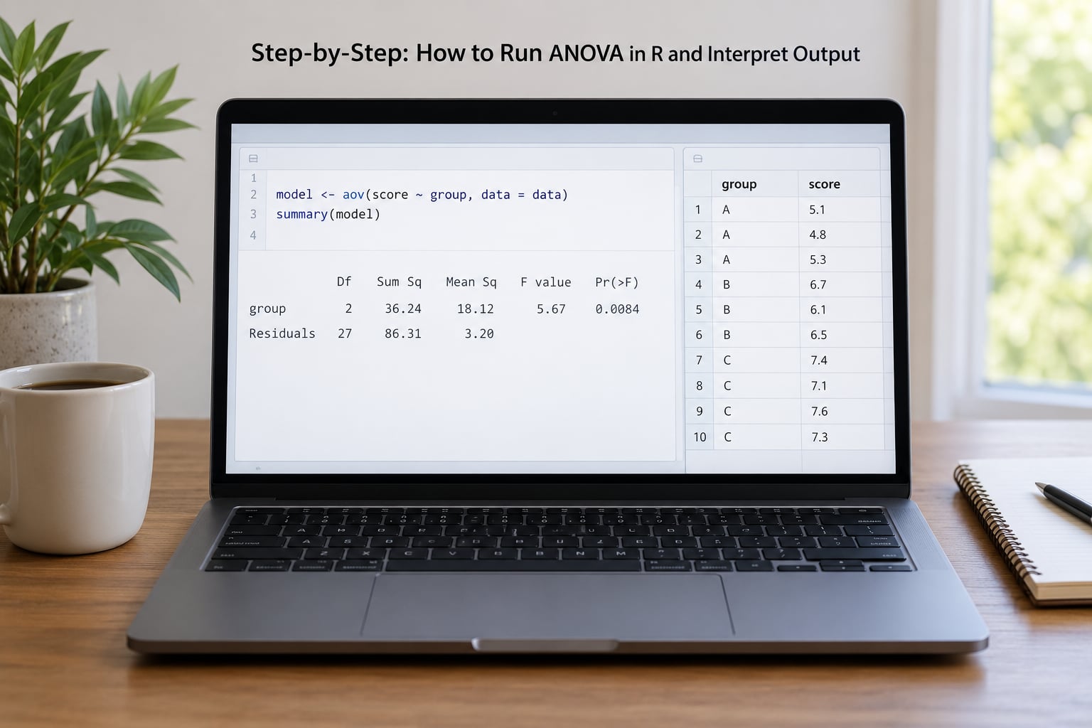
The dataset is exam scores from 30 students, ten per teaching method: lecture, group work and blended. Scores run roughly 58 to 92. You want to know whether the average score differs across the three methods.

Step 1: Prepare and Inspect the Data

Start by confirming the outcome is numeric and the group column is a factor.

str(mydata)
'data.frame':	30 obs. of  2 variables:
 $ method : Factor w/ 3 levels "Lecture","Group Work","Blended": 30
 $ score : num  68 74 79 75 84 71 66 77 82 70 ...

The word Factor in that output is what you want. If it says int or num instead, your group labels are numeric and you convert them:

mydata$method <- factor(mydata$method)

Check the levels and counts so you know the groups are spelled consistently. A stray space in “Group Work” creates a fourth empty group.

table(mydata$method)

    Lecture Group Work    Blended
        10         10        10

Ten per group, and none of the counts is zero. That is what successful preparation looks like.

Look at the group means and standard deviations before you test anything. If one group’s mean sits far away from the others, you already have a hint of what the result will say.

tapply(mydata$score, mydata$method, mean)
tapply(mydata$score, mydata$method, sd)
tapply(mydata$score, mydata$method, length)

    Lecture  Group Work     Blended
70.4        80.9        75.0
 6.2         5.8         6.5
   10         10          10

Now check for missing values, because aov() silently drops rows with NA, and if a whole group loses rows your result changes.

sum(is.na(mydata$score))
[1] 0

Zero here. If the number is not zero, use complete.cases() or na.omit() and report how many observations you removed.

Step 2: Check the ANOVA Assumptions

ANOVA assumes independent observations, roughly normal residuals within each group, and equal variances across groups. You check the last two, and you reason about the first from your study design.

Fit the model first, because the assumption checks all use the fitted residuals.

fit <- aov(score ~ method, data = mydata)

For normality, the base R diagnostic plots are the fastest look. Four plots in one window: residuals against fitted, scale-location, normal Q-Q, and residuals against leverage.

par(mfrow = c(2, 2))
plot(fit)

The points in the Q-Q plot should sit close to the straight line. A pronounced curve or one or two far-off points suggests non-normal residuals. The residuals-versus-fitted plot should show an even band of points around zero with no funnel or curve. A funnel shape usually points to unequal variances rather than non-normality.

You can back the visual read with a formal test. The Shapiro-Wilk test works on residuals, not on the raw scores:

shapiro.test(residuals(fit))

	W = 0.981
	p-value = 0.628

For equal variances, Bartlett’s test is built into base R.

bartlett.test(score ~ method, data = mydata)

	Bartlett test of homogeneity of variances
	data:  score by method
	Bartlett's K = 0.86
	df = 2
	p-value = 0.65

The car package gives you Levene’s test, which is less sensitive to departures from normality. Install it once with install.packages("car"), then:

library(car)
leveneTest(score ~ method, data = mydata)

Levene's test for homoscedasticity of central location
data:  score by method
Levene's Chi-Sq on df =  2 gives p-value = 0.42

A p-value below .05 on either variance test means the homoscedasticity assumption is in trouble. That does not mean you abandon the analysis. Switch to Welch’s ANOVA, which does not assume equal variances:

oneway.test(score ~ method, data = mydata)

	One-way analysis of variance by Welch

data:  score and method
F = 7.27, num df = 2.0, denom df = 25.5, p-value = 0.004

Reading the same p-value from Welch’s version is normal. Small differences in p come from the fractional degrees of freedom, not from an error.

Step 3: Run the ANOVA Model

The full call is one line. The formula reads “outcome depends on group”, and data = mydata tells R where to find those columns.

fit <- aov(score ~ method, data = mydata)
summary(fit)

The equivalent long form is anova(lm(score ~ method, data = mydata)). Both build the same linear model, and aov() is just the tidy wrapper. Many packages expect a model object from lm(), so keep that version in mind if a later function rejects fit.

Confirmation that the model fitted is the summary() block printing the ANOVA table. If nothing appears, the model did not build, and you need to read the error message rather than guess.

Step 4: Interpret the ANOVA Output

Here is the whole output for the example.

> summary(fit)
             Df    Sum Sq   Mean Sq   F value  Pr(>F)
method        2   554.06    277.03     7.27   0.0030 **
Residuals    27  1028.97     38.11
---
Signif. codes:  0 '***' 0.001 '**' 0.01 '*' 0.05 '.' 0.1 ' ' 1

Two rows. The first row, method, holds the variability explained by group membership. The Residuals row holds everything the model could not explain, which is the spread of scores inside each group.

Column by column:

Column	What it means	Read it as
Df	Degrees of freedom, the number of independent pieces of information left after the model is fitted	2 between groups because 3 groups minus 1; 27 within because 30 observations minus 3 group means
Sum Sq	Sum of squares, the total squared spread attributable to that source	554.06 is between-group spread; 1028.97 is leftover spread
Mean Sq	Sum Sq divided by Df, which puts both rows on the same scale	277.03 versus 38.11
F value	The F ratio: between-group mean square divided by within-group mean square	277.03 / 38.11 = 7.27. Values near 1 mean the groups look alike; values well above 1 mean the groups are separated
Pr(>F)	The p-value: the probability of seeing an F this large if all group means were truly equal	0.0030 is below .05, so the null hypothesis is rejected
Signif. codes	The star legend printed at the bottom	Two stars means p is below .01

Two stars on the p-value means p is smaller than .01. One star is below .05, a dot is below .10, three stars is below .001. Reading the legend once saves you guessing later.

The null hypothesis is that all three population means are equal. Rejecting it means at least one group mean differs from at least one other. It does not say which pairs differ, and it does not say how large the difference is.

The Residuals row has no F value and no p-value by design. It is the denominator of the F ratio, the baseline noise you compare against. Nothing is tested against it.

If Pr(>F) comes back at 0.42 instead, the honest reading is that the data do not give you enough evidence to rule out equal means. That is a statement about evidence, not proof of similarity. With only ten students per group, a real difference of a few points can easily go unnoticed.

Step 5: Identify Which Groups Differ

A significant omnibus test does not tell you which groups differ, and this is the most common reporting mistake I see. You need a post-hoc comparison, which controls the family-wise error rate across all pairs.

TukeyHSD(fit)

	Tukey multiple comparisons of means
    95% family-wise confidence intervals

$method
                diff    lwr    upr p adj
Group Work-Lecture  10.50  0.75 20.25   0.02
Blended-Lecture      4.60 -5.15 14.35   0.35
Blended-Group Work  -5.90 -15.65  3.85   0.21

Read the p adj column, not the raw differences. Adjusted p below .05 means that pair differs after accounting for the other comparisons. Here, group work scores higher than lecture by 10.5 points with an adjusted p of .02, while blended differs from neither. The confidence interval from 0.75 to 20.25 makes that concrete.

The alternative route is pairwise.t.test() with an explicit adjustment:

pairwise.t.test(mydata$score, mydata$method,
                p.adjust.method = "holm")

Never run pairwise.t.test() without the adjustment argument. With four groups you would be running six unadjusted tests, and the chance of at least one false positive climbs well above 5 percent.

For Welch’s model, use Games-Howell instead, because Tukey’s intervals assume equal variances:

library(PMCMRplus)
gh <- gamesHowellTest(score ~ method, data = mydata)

Step 6: Calculate Effect Size and Report the Result

The p-value answers whether a difference is likely real. It says nothing about whether the difference is worth acting on. With a large enough sample, a two-point difference becomes significant, which is why you report an effect size alongside it.

Eta squared is the proportion of total variability in the outcome explained by group membership. One line of base R gives it:

summary(fit)[[1]][1, "Sum Sq"] / sum(summary(fit)[[1]][, "Sum Sq"])
[1] 0.3501

Eta squared of .35 means about 35 percent of the variation in exam scores is accounted for by which method a student was taught with. A rough guide: .01 is small, .06 is medium, .14 is large. Omega squared is a less biased version, and here it comes out around .29.

The APA sentence reports the test, the degrees of freedom, the F, the p-value and the effect size:

A one-way ANOVA showed a significant effect of teaching
method on exam score, F(2, 27) = 7.27, p = .003, omega
squared = .29. Tukey HSD post-hoc tests showed that group
work (M = 80.9) scored significantly higher than lecture
(M = 70.4), while blended (M = 75.0) did not differ
significantly from either.

For a nonsignificant result the sentence reads differently: “A one-way ANOVA indicated no significant difference in exam score by teaching method, F(2, 27) = 1.5, p = .23, omega squared = .01.” Report it. Leaving it out invites the question of whether you ran the test at all.

Common Mistakes

• Group labels coded as numbers. If the method column holds 1, 2 and 3, R treats it as a continuous predictor and returns a one-df test comparing a straight line through the data. Fix: mydata$method <- factor(mydata$method). A correct one-way ANOVA on three groups always shows Df = 2 on the factor row.
• Wide-format data. One column per group gives you a test per column and no omnibus result. Fix: reshape to long format before fitting.
• Reading a significant F as “every group differs”. It only says at least one pair differs. Fix: always run Tukey HSD or Games-Howell and report the pairs.
• Treating p below .05 as proof of a large effect. Fix: report eta squared or omega squared next to the F and p.
• Ignoring a failed assumption check. Fix: switch to Welch’s ANOVA for unequal variances, or to Kruskal-Wallis for badly skewed data. Neither is a failure, both are standard.
• Misreading the degrees of freedom. For k groups and n total observations, Df between is k minus 1 and Df within is n minus k. Welch’s test reports fractional denominator df, which is normal, not a bug.
• Reporting only the p-value. Fix: include F, both df values, p and an effect size so the result is usable by someone who never saw your console.

Frequently Asked Questions

Conclusion

Start by checking your variables: is the outcome numeric, is the grouping column a factor, and are the counts per group what you expect. Then inspect the assumptions, fit the model with aov(), and read the F value and Pr(>F) alongside an effect size rather than on their own.

That is the whole of how to run ANOVA in R and interpret output. The next practical step is to run Tukey HSD on any significant result and write the APA sentence with the F statistic, both degrees of freedom, the p-value and the effect size in one place.