What to Do With Outliers in Statistical Analysis (2026)

An outlier is an observation whose value sits far enough from the rest of the data to distort the mean, the standard deviation or a fitted model. What to do with outliers in statistical analysis comes down to one question: is this value wrong, rare but real, or simply pulling hard on your answer?

There are four defensible treatments. Keep the value if it is real. Remove it only if you can prove it is an error. Transform or winsorize it if the distribution is the problem. Switch to a method that is not driven by extreme values if the parameter is the problem. Everything below is a workflow for choosing between those four, and for writing down why you chose.

Nobody gets in trouble for reporting an outlier. They get in trouble for deleting one without a reason.

Table of Contents

1. 1What You Need
2. 2Step-by-Step: What to Do With Outliers in Statistical Analysis
3. 3What to do with outliers in statistical analysis: start by defining the observation
4. 4Check the data for entry and processing errors
5. 5Identify outliers using plots, rules, and residuals
6. 6Determine whether the observation changes the analysis
7. 7Choose and justify the appropriate treatment
8. 8Re-run diagnostics and report the decision
9. 9Common Mistakes
10. 10Frequently Asked Questions
11. 11Should outliers always be removed from a dataset?
12. 12What rule should I use to identify an outlier?
13. 13Are outliers necessarily errors or missing data codes?
14. 14How should I handle outliers when my sample is small?
15. 15Should I use the IQR rule, z-scores, or residual diagnostics?
16. 16How do I report outlier decisions in a research paper?
17. 17Conclusion

What You Need

Before you touch a single case, have these five things lined up. Missing any of them is how analysis goes wrong quietly.

• The prepared dataset, with the analysis variable already coded the way the plan says it should be.
• Variable definitions and the codebook, including the units, the valid range and any recorded missing-value codes such as 999 or -99.
• Access to the source records — the questionnaire, the lab sheet, the export log — because verification is impossible without them.
• The research question and the model you chose. An outlier is relative to a model, so “outlier” is not a property of the number alone.
• Diagnostic output: a histogram, a box plot, a scatter plot, and the residual plots from your fitted model.
• Software. Everything in this guide runs in R, Python, SPSS or Stata. Pick the one your lab already uses so the code is reproducible by someone else.

Step-by-Step: What to Do With Outliers in Statistical Analysis

The workflow below moves in a fixed order: define, verify, identify, test, treat, report. Skipping straight to treatment is what produces unreproducible papers.

What to do with outliers in statistical analysis: start by defining the observation

Three different things get called an outlier, and they need different treatments. Sorting them out first saves you from deleting a valuable case.

A data error. A weight recorded as 950 pounds, a survey coded 5 when the respondent picked 2, a decimal point in the wrong place. This is not an outlier in any interesting sense. It is a mistake, and mistakes get corrected or removed.

A legitimate extreme value. A 19-year-old in a study of retirement savings. A 340-millisecond reaction time in a well-rested participant. A spike in monthly electricity use during a heatwave. The value is real, and it belongs in the analysis because your population genuinely contains cases like it.

An influential observation. This one surprises people: an observation can sit comfortably inside the bulk of the data and still change your slope, your p-value or your conclusion. Influence is about effect on the fit, not about distance from the mean.

Related but separate: a leverage point sits far from the centre of the predictors, so it has unusual power over the fitted line even if its residual is small. An observation can be an outlier in y, an outlier in x, influential, or any combination.

Check the data for entry and processing errors

This is the step that most people skip, and it is the one that catches the most real problems. Work through it before you compute a single flag.

1. Check units and decimal placement. Sort the variable and read the top ten values aloud. Does a 340-millisecond value sit next to 0.34-second values?
2. Check missing-value codes. Any 999, 888 or -99 left in the numeric variable will be flagged as an outlier by every rule you apply. Convert them to true missing values first.
3. Check duplicates. A record entered twice can look like a legitimate pair of extremes, especially in a small sample.
4. Check impossible values. A percentage over 100, an age under 0, a score outside the scale range. Compare against the scale definitions in your codebook.
5. Check the merge and the transformations. Reversed coding, a subtracted constant in the wrong direction, or a merge that pulled records from the wrong study period all produce textbook outliers.
6. Check the source. For any case that still looks wrong, go back to the original questionnaire or instrument. If the source says the value is right, stop hunting for an explanation.

If step six finds a mistake, correct it from the source and record the change. Do not simply delete the row.

Identify outliers using plots, rules, and residuals

Look first, then compute. Plots tell you about shape and multimodality in a way no single number does.

A histogram shows skew and whether you have two populations in one variable. A box plot shows the quartiles and any tail that stretches past the whiskers. A scatter plot shows whether the extreme point is off the relationship or simply at the edge of it.

After that, the numeric rules:

Method	What it assumes	Best for	Typical flag
Z-score (3-sigma)	Roughly symmetric, mean-centred data	Quick screening of a near-normal variable	|z| > 3
1.5 x IQR rule (Tukey)	Median and quartiles, which resist extreme values	Skewed data and box plots	Beyond Q1 – 1.5(IQR) or Q3 + 1.5(IQR)
Grubbs’ test	One outlier, normally distributed data	Small samples where you want a formal test	G above the critical value at your alpha
Rosner’s generalized ESD	Nearly normal data, several outliers	Datasets where more than one case may be extreme	Significant ESD at k outliers
Studentized residual	A fitted model is correct apart from the case	Regression and ANOVA, where “outlier” is model-relative	|r| > 2 to 3
Cook’s distance	Only a linear model	Finding influential cases, not just odd ones	D > 4/n, or D > 1
Leverage (hat value)	Only a linear model	Finding cases that are extreme on the predictors	h > 2p/n or 3p/n
Mahalanobis distance	Covariance is estimable	Multivariate outlier cases across several variables	Top percentile of the chi-square distribution

Two cautions about these numbers. First, every threshold is a diagnostic aid, not an automatic deletion rule; a case outside 1.5 IQR is a reason to look, not a reason to delete. Second, the IQR fence itself moves when you remove cases, so re-running the rule after a deletion gives you a different answer than the first run. Decide your rule before you look at the results, and write it down.

A note on z-scores, since it comes up constantly: with a sample large enough for a z-score to be meaningful, |z| = 2.5 is not unusual. Roughly two percent of normally distributed observations sit beyond two standard deviations. Values between 2 and 3 are worth noting, not deleting.

Determine whether the observation changes the analysis

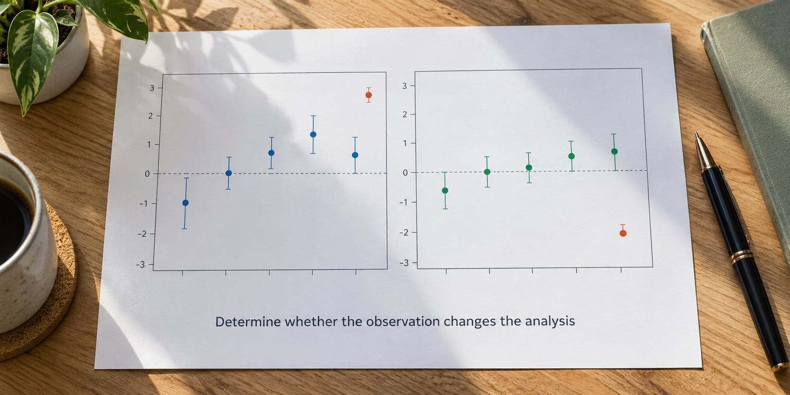
Now do the thing that actually answers the question: refit your model with and without each flagged case and compare. If the estimate barely moves, the case is not worth a fight with your supervisor.

A large residual with low influence means the observation is odd but not doing damage to the fit. A small residual with high influence means the opposite, and that is the dangerous case: it sits quietly inside the data while dragging your slope toward it. Cook’s distance exists to catch precisely this situation.

Compare the estimates, the standard errors, the confidence intervals and the p-values across the two runs. If the sign of your main effect flips, or the significance crosses 0.05, you have an influential observation and a decision to make, not a cleanup task.

This is also the moment to ask whether a resistant method would tell you the same story. Quantile regression, median regression or an M-estimator fit such as a Huber loss produces an estimate that one extreme value cannot dominate. If that estimate agrees with the trimmed-sample result, your conclusion is not fragile.

Choose and justify the appropriate treatment

Pick from these six, in this order of preference.

1. Correct the error. A verified data-entry mistake is fixed from the source document. Record the original and corrected values.
2. Keep it. The right answer for a rare but real value, and the default whenever you cannot prove otherwise. Practitioner consensus on r/AskStatistics and r/labrats is consistent on this: remove only when the case causes a false positive or is clearly a mistake.
3. Exclude it under a predefined rule. Permissible when the exclusion criterion was written into the protocol or analysis plan before you saw the data, and applied uniformly to all cases. Choose winsorizing instead if you also need to preserve your sample size.
4. Transform the variable. A log, square root or Box-Cox transformation compresses the tail and can remove the need to delete anything. Back-transform carefully for any descriptive statistics you report.
5. Use a method that resists extreme values. Quantile regression, median regression, trimmed means, bootstrap standard errors, or an M-estimator. This keeps every observation and usually changes the estimates less than deletion does.
6. Model the structure instead. If the extreme values belong to a second population, fit separate groups, test the group effect, or allow a nonlinear or segmented relationship. Collapsing two groups into one variable is what manufactured the outlier in the first place.

Here is the same logic in code, so the decision is reproducible rather than remembered.

R — flag by IQR and by studentized residual:

# IQR fences
q <- quantile(x, c(0.25, 0.75))
iqr <- q[2] - q[1]
flag <- x < q[1] - 1.5 * iqr | x > q[2] + 1.5 * iqr

# model-relative outliers in a linear model
fit <- lm(y ~ x)
which(abs(studentresid(fit)) > 2)
which(cooks.distance(fit) > 4 / length(y))

# a fit that one extreme point cannot dominate
qreg(y ~ x, quantile = 0.5)

Python:

import numpy as np
from statsmodels.robust.robust_linear_model import RLM

q1, q3 = np.percentile(x, [25, 75])
iqr = q3 - q1
flag = (x < q1 - 1.5 * iqr) | (x > q3 + 1.5 * iqr)

ols = sm.OLS(y, X).fit()
print(ols.get_influence().summary_frame()["cooks_d"])

# median-style fitting keeps every observation
resistant = RLM(y, X).fit()

SPSS: use Analyze > Descriptive Statistics > Explore, then in the Statistics box tick Outliers (5%) for Tukey’s 1.5 IQR fences and Percentiles. For regression, request Residuals > Studentized in Regression > Residual plots and check the scatterplot of standardized residual against predicted value.

Stata:

quietly summarize price
local q1 = r(p25)
local q3 = r(p75)
local iqr = `q3' - `q1'
gen flag = price < `q1' - 1.5*`iqr' | price > `q3' + 1.5*`iqr'
reg y x
predict double sr, studentized
predict double cd, cooksd
qreg y x, quantile(0.5)

Re-run diagnostics and report the decision

After any treatment, run the diagnostics again. A transformation changes the residuals, so check normality and homoscedasticity on the transformed scale, not the original one. If you removed cases, look at what the new box plot does; if you winsorized, confirm the tail is now bounded rather than absent.

Then write it up. A reviewer should be able to reconstruct your decision from four sentences:

1. The rule. The criterion you used, ideally fixed in advance.
2. The method. The named detection method and threshold.
3. The count and the effect. How many cases were affected, and what happened to the estimates, confidence intervals and p-values with and without them.
4. The final decision and the audit trail. What you did, plus a sensitivity analysis showing that the conclusion holds under the alternative.

Report the with-and-without comparison even when the conclusion does not change. That single sentence is what separates defensible outlier treatment from accusations of data dredging, and it is the part students most often leave out.

Common Mistakes

These seven account for most of the bad outlier decisions I have seen reviewed. Each has a straightforward fix.

• Deleting everything the rule flags. A 1.5 IQR rule on 500 mildly skewed values can flag 5 percent of the sample by itself. Fix: treat flags as review candidates, not verdicts.
• Choosing a threshold after seeing which one gives significance. This is selection on the outcome, and it invalidates the test. Fix: fix alpha and the method in the protocol, then report.
• Using one rule for every variable. Income and a 7-point Likert scale do not belong in the same rulebook. Fix: match the method to the distribution and the scale.
• Ignoring group structure. Two clusters combined make one cluster look extreme. Fix: plot by group, and test for group differences before flagging within groups.
• Skipping the sensitivity check. If you never refit without the case, you do not know whether it mattered. Fix: always run both and record both.
• Documenting too little. “Two outliers were excluded” is not reproducible. Fix: give the rule, the count, the method and the effect on the estimates.
• Treating a real rare case as noise. Genuine extreme values often carry the effect you are looking for. Fix: prefer keeping, winsorizing or resistant estimation over deletion.

One more worth naming: on r/labrats and r/statistics, the recurring advice is to think carefully before removing anything, because the default should be retention. That is not timidity. It is the position that survives review.

Frequently Asked Questions

Conclusion

Start by verifying the observation, not by deleting it. Check the codes, the units and the source record, because most flagged values turn out to be either a coding mistake or a real case that happens to be rare.

Then work through the sequence in order: identify with a method that suits your data and model, test whether the case actually changes the answer, choose the mildest treatment that solves the problem, and re-run your diagnostics. A transformation, winsorizing or a resistant estimator usually fixes an analysis that a deletion would break.

Your first move is cheap: run a box plot and a residual check today, before you commit to anything. Whatever you decide, write down the rule, the method, the count and the before-and-after estimates. That paragraph is what turns a debatable analysis into a defensible one.