How to Classify Land Cover in Remote Sensing Software in 2026

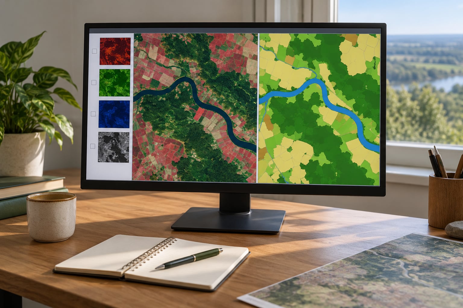
Land cover classification is the process of sorting every pixel in a satellite or aerial image into a category such as water, forest, short vegetation, agriculture, bare soil or built-up land. To classify land cover in remote sensing software, you define your classes, prepare the imagery, label a set of representative samples, run a classifier and then check the result against ground truth you held back. Budget a weekend for a small study area and a couple of weeks if your reference data has to be collected from scratch.

Most beginner maps fail for the same reason: the classes were never defined carefully, or the accuracy figure came from the same samples used to train the model. Both are fixable, and both are explained below.

Table of Contents

1. 1What You Need
2. 2Step-by-Step
3. 31. Define the Land-Cover Classes
4. 42. Prepare and Inspect the Imagery
5. 53. Select Software and a Classification Approach
6. 64. Collect Training and Reference Data
7. 75. Train the Land-Cover Classifier
8. 86. Validate the Classification Map
9. 97. Export and Document the Final Result
10. 10Common Mistakes
11. 11Frequently Asked Questions
12. 12What are the different classifications of land cover?
13. 13What is a land cover type?
14. 14Are land cover and land use the same?
15. 15What is the difference between supervised and unsupervised classification?
16. 16How many training samples per class do I need?
17. 17What is a good overall accuracy for a land cover map?
18. 18How do I convert a classified raster to polygons?
19. 19Conclusion

What You Need

Before opening any software, get four things straight. Everything downstream gets easier when these are settled.

Imagery. A scene that covers your study area with as little cloud as possible, acquired in the season your land cover is most stable. For most coursework that means Landsat 8 or 9 Collection 2 at 30 m, or Sentinel-2 at 10 m when you need finer boundaries. Both are free to download once you have an account with USGS EarthExplorer or the Copernicus Browser.

Class definitions. A written list, before you look at pixels, of what each class means and what it excludes. “Built-up” needs a decision: does a single house in a field count, or does a class need a continuous footprint? Ambiguity here is the root cause of most class confusion later.

Reference data. Points or polygons whose true class you know, used for training and, separately, for validation. Field GPS tracks, a national land-cover dataset such as the USGS National Land Cover Database (NLCD) or ESA WorldCover, or your own interpretation of high-resolution aerial imagery all qualify. What you cannot do is use the same polygons for both.

Software. Any desktop or cloud GIS with a supervised or unsupervised classification tool. QGIS with the Semi-Automatic Classification Plugin (SCP) is the most common free route, Google Earth Engine handles large areas without downloads, and SNAP, the Orfeo Toolbox, ArcGIS Pro, ENVI and ERDAS Imagine all work.

Project requirements. Check what your course, paper or agency actually asks for: number of classes, required accuracy reporting, a specific class scheme, or a vector rather than raster output. Building to that spec from the start is cheaper than reworking a finished map.

Step-by-Step

The workflow below is the order that produces a defensible land-use and land-cover (LULC) map. It is identical in principle across QGIS, SNAP, Earth Engine, ENVI and ArcGIS Pro, even though the menu names differ.

1. Define the Land-Cover Classes

Start from the question, not from a legend someone else published. If your study is urban expansion, built-up needs to be split into built-up and bare soil; if it is watershed characterisation, impervious surface and forest may matter more than cropland.

Three rules keep a class list workable. Classes must be mutually exclusive, so no pixel can reasonably be assigned two of them. They must be spectrally separable at your resolution, meaning different classes should not look identical in a false-colour composite. And they must be definable on the ground, because at some point a stranger with your legend has to label a pixel the same way you did.

Match the smallest class to the pixel size. A 30 m Landsat pixel covers 900 square metres, just under a tenth of a hectare, so anything narrower than a large building is invisible; a class defined as “parking” on 30 m imagery is a class you cannot map, no matter how good the classifier is.

Class	Typical spectral behaviour	Often confused with	NLCD / ESA WorldCover equivalent
Water	Very low reflectance in all visible and near-infrared bands	Deep shadow, dark asphalt	Open Water / Water
Tree cover	Moderate visible, high near-infrared response	Short vegetation, dense crop canopy	Deciduous and Evergreen Forest / Tree Cover
Short vegetation	Moderate to high reflectance across visible and near-infrared	Cropland, tree cover in dry season	Shrubland, Grassland / Grassland
Cropland	Green to yellow seasonal pattern, regular field boundaries	Grassland, bare soil after harvest	Cropland, Pasture / Cropland
Bare soil	High visible reflectance, low near-infrared	Urban rooftops, sand, dry riverbed	Barren Land / Bare and sparse vegetation
Built-up	Irregular across all bands, high variance within class	Bare soil, quarries, industrial sites	Developed classes / Built-up

Six to eight classes is a sensible ceiling for a first map. Adding a ninth barely changes overall accuracy but makes every training sample harder to collect.

2. Prepare and Inspect the Imagery

Download the scene and open it before doing anything else. Look at it in a false-colour composite (near-infrared in red, red in green, blue in blue for most sensors) so vegetation, bare ground and built-up separate visually. If you cannot tell those apart by eye, a classifier will not either.

Check spatial and spectral resolution against your class list. A 10 m Sentinel-2 scene lets you separate narrow roads and small water bodies that Landsat merges into mixed pixels. It also brings more noise, so band selection matters more.

Preprocessing is not always mandatory, and over-processing is a real mistake. Atmospheric correction (for example the dark object subtraction or LaSRC-style corrections, or the Sen2Cor algorithm for Sentinel-2) helps if you are comparing reflectance values across scenes or dates. Cloud and shadow masking is close to mandatory, because a thin cloud edge looks enough like bare soil or built-up to poison a class.

Clip the scene to your area of interest to cut file size and processing time. Do this in the same coordinate reference system you will use for the final map, and record what it is. Mixing a UTM projection with WGS84 layers is a reliable source of shifted training polygons that never quite line up with the imagery.

3. Select Software and a Classification Approach

Two decisions here drive everything else: supervised or unsupervised, and which tool. Neither has a universally correct answer, so pick based on the study area and the resources you actually have.

Supervised classification uses samples you have labelled. You say “these 40 pixels are forest” and the algorithm works out the rule, then applies it to the rest. It gives you class names you control, which is why it is the default for any map that has to be explained to someone.

Unsupervised classification lets a clustering algorithm (k-means, isodata, mean shift, or the K-means clustering available in most tools) find natural groupings of pixels first. You then label the clusters afterwards. It is fast, needs no ground data, and works well on a study area you have never seen before.

Hybrid runs clustering first, labels the clusters, then re-runs a supervised classifier with those labels as training. It is more work but it consistently beats either method alone when your classes are spectrally messy.

Approach	You supply	Strengths	Weaknesses	Use it when
Supervised	Labelled training polygons	You control class names and boundaries; validation is straightforward	Slow to prepare; biased by your own interpretation	You know the area, or have reference data
Unsupervised	Number of clusters	Fast, no ground data needed, good for exploration	Clusters rarely match your class list; needs manual labelling	Exploring an unfamiliar area, or when reference data is thin
Hybrid	Cluster labels plus refinement	Better separation, easier to refine iteratively	Longest workflow; two places for errors to hide	Spectrally similar classes need separating

On the software side, here is how the common options actually differ.

Software	Cost	Learning curve	Batch automation	Accuracy tools	Best for
QGIS + Semi-Automatic Classification Plugin	Free and open source	Moderate	Python console and processing models	Confusion matrix, classification report	Students and small desktop projects
Google Earth Engine	Free, cloud-based	Moderate to steep (JavaScript or Python)	Excellent, built in	Confusion matrix and Kappa in code	Continental or multi-year work with no downloads
ESA SNAP	Free	Steep	Good, command line and graph builder	Vector and raster confusion matrices	Sentinel and other ESA missions
Orfeo Toolbox	Free	Steep	Good	Confusion matrix via OTB applications	Research pipelines and large time series
ArcGIS Pro	Commercial, academic licences available	Moderate	ModelBuilder, Python, geoprocessing history	Confusion matrix, accuracy assessment tool	Coursework requiring Esri deliverables
ENVI	Commercial	Steep	IDL scripting	Classification tools with report output	Hyperspectral data such as AVIRIS or Hyspec
ERDAS Imagine	Commercial	Steep	Spatial Modeler	Classification and accuracy reports	Legacy coursework and long-standing workflows
R (terra, randomForest) or Python (rasterio, scikit-learn)	Free	Steep, needs coding	Total control, versioned and repeatable	Whatever you write, which is the point	Reproducible research and publication figures

The QGIS community treats the Semi-Automatic Classification Plugin as the most accessible free route for Landsat work, and the plugin’s own manual remains the canonical reference for its tools. Earth Engine has become the default for large-area processing because Random Forest runs there without downloading a single scene, usually through the geemap Python package.

Whichever route you take, pick one and stay there long enough to learn where training, classification and accuracy live. Switching tools halfway through a project is the most common way people lose a week.

4. Collect Training and Reference Data

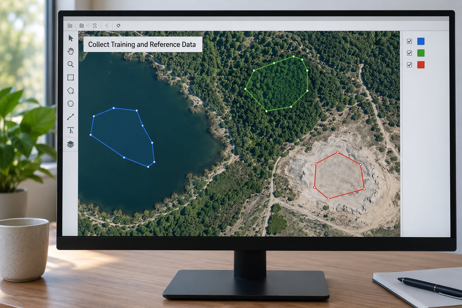
This is the step people underestimate, and it is where most maps are won or lost. Drawing training data is slow because it requires actual interpretation, not clicking.

Use polygons rather than single pixels wherever the software allows it. A polygon gives the classifier many pixels to learn from and reduces the chance that one shadowed tree defines your whole forest class.

On quantity, the community rule of thumb is generous: aim for roughly 50 to 100 reasonably sized polygons per class, and draw them spread across the whole study area rather than concentrated in the easiest spot. Small, homogeneous classes such as water can get by with fewer; heterogeneous ones such as built-up need far more because the class contains dark roofs, bright roofs, roads and shadow, and a training set that only contains dark roofs will label everything else wrong.

Four habits keep samples honest:

• Spread them. If your cloud-free study area is 20 km across, do not train on one corner. Include the outskirts, the river valley and the hills.
• Vary within classes. Deliberately sample built-up in the city centre and in a village, forest in dense and sparse stands.
• Stay inside the class. A polygon that clips a tree line teaches the classifier that edge is fine. Keep mixed pixels out unless you are deliberately building a mixed class.
• Keep a validation set separate. Draw extra reference polygons or collect GPS points, then never use them for training.

That last point deserves emphasis. If you validate with the training data, you get resubstitution accuracy, which measures how well the model memorised itself and is routinely 15 to 25 points higher than the truth. Users on QGIS and ArcGIS community forums describe building a confusion matrix from an external ground-truth file as fiddly, and the workaround is worth the effort: create a separate point layer with a class field, then use it as the validation reference in the accuracy tool.

For every reference point or polygon, record where it came from and when: the survey date, the GPS accuracy, or the dataset name and release year. A land-cover map from imagery acquired in June and validation points from an older survey is not a small detail to leave out of a paper.

5. Train the Land-Cover Classifier

With samples in place, choose features and set the model up. Which classifier to use depends more on your data than on any ranking.

Classifier	How it works	Strengths	Weaknesses	Use it when
Maximum likelihood	Assumes class spectra are normally distributed and picks the most likely class per pixel	Fast, classic, widely taught	Strict assumptions; fails on non-normal distributions	A course or exam that expects the standard method
Minimum distance	Picks the class whose mean spectrum is closest	Very fast, minimal assumptions	Ignores class variance	Quick look, or a first sanity check
Support vector machine	Finds the boundary that separates classes with the widest margin	Strong with limited, clean samples	Slow on very large scenes; sensitive to sample placement	Few hundred good samples, many bands
Random forest	Builds hundreds of decision trees and averages their votes	Handles noise and nonlinear class overlap; resists overfitting	Less interpretable; slower than MLC	Most real projects, especially confusable classes
Spectral angle mapper	Compares the angle between pixel and class spectra	Insensitive to overall brightness, good for shaded data	Weak with similar spectra	Imagery with strong illumination differences
K-means or isodata clustering	Groups pixels into clusters without labels	No training data needed	Clusters are not classes until you name them	Exploration, or as the first stage of a hybrid run

Random Forest is the pragmatic default for a beginner’s final map, because it keeps a high accuracy even when two classes overlap spectrally. Keep maximum likelihood in your back pocket when a supervisor expects it.

On features: start with the reflectance bands only, and add spectral indices such as NDVI or NDWI one at a time so you can see whether each helps. Feeding every band and index into a small training set is a common way to overfit.

Watch class balance. A class with 2,000 training pixels and a class with 40 will be over-predicted. Bring the counts closer together, or set class weights if the tool offers them.

Then read the output rather than just saving it. Concrete signs the run needs another pass:

• Single scattered pixels inside a large homogeneous block, or the familiar salt-and-pepper speckle.
• A class that has swallowed its neighbour, typically grassland labelled cropland.
• Whole classes missing entirely, which usually means those classes never got labelled in the training set.
• A visible boundary that follows the edge of your training data, which means polygons too large or too few.

Fix the cause rather than the symptom. Adding samples to the starved class, splitting built-up into impervious and non-impervious, or removing mixed edge pixels usually does more than any classifier setting.

6. Validate the Classification Map

Accuracy assessment is the part students skip, and it is the part that decides whether your map is defensible. The method is standard: build a confusion matrix comparing your map against independent reference data.

Each cell of the matrix is a count of pixels the map assigned to one class when the reference said another. Every accuracy metric is derived from those counts.

Metric	What it measures	How to read it
Overall accuracy	Share of all validation pixels classified correctly	A headline number, but it hides which classes are failing
Producer’s accuracy	How complete a class is	PA = 100% minus omission error; how much of the real class you found
User’s accuracy	How reliable a class label is	UA = 100% minus commission error; how much of what you labelled is correct
Kappa coefficient	Agreement corrected for chance	Above 0.8 is strong, 0.6 to 0.8 moderate, below 0.4 little better than random

On what counts as acceptable: community reports from beginner land cover projects cluster around 75 to 85 percent overall accuracy, and that range is a reasonable target for a first supervised map with six or seven classes at 30 m. Going much higher often means the classes are too easy or the validation data is not truly independent. Going below 70 percent usually points at training data, not at the classifier.

Always report per-class numbers alongside the overall figure. A map at 80 percent overall can still have 45 percent producer’s accuracy for cropland, and that is the number a reviewer will ask about.

Report honestly, too. State your imagery, its acquisition date, the software and version, the classifier, the number of samples per class, and how validation points were collected. Anyone reproducing your map needs all of it.

7. Export and Document the Final Result

Export twice: a GeoTIFF raster for analysis and a vector polygon layer for anyone who will use the map in a planning document. Converting raster to vector, in QGIS through Polygonize, or in ERDAS and ENVI through their vectorize tools, is straightforward, but set a minimum mapping unit first. Without one, you get thousands of single-pixel polygons from the speckle you never cleaned up.

Clean before you vectorize. A modal or majority filter (GRASS’s r.to.vect after r.filter.mode, or the equivalent tool in your software) over a 5 by 5 window removes isolated pixels while leaving real boundaries intact. Do it before converting, and keep the unfiltered raster so anyone can check what the filter removed.

Preserve your class labels as integer values with a fixed palette and a written legend. Values that change meaning between a QGIS session and an ArcGIS one cause a lot of confusion.

Document the run: software name and version, plugin version, classifier and its settings, band list, class codes, the number of training samples per class, filter window size, and if your classifier uses one, the random seed. Changing the seed can move your accuracy by a point or two, so record it or your results will not replicate exactly.

If you intend to publish, attach provenance: source scene identifiers, processing steps, and the validation table. That is what separates a defensible map from a picture of a map.

Common Mistakes

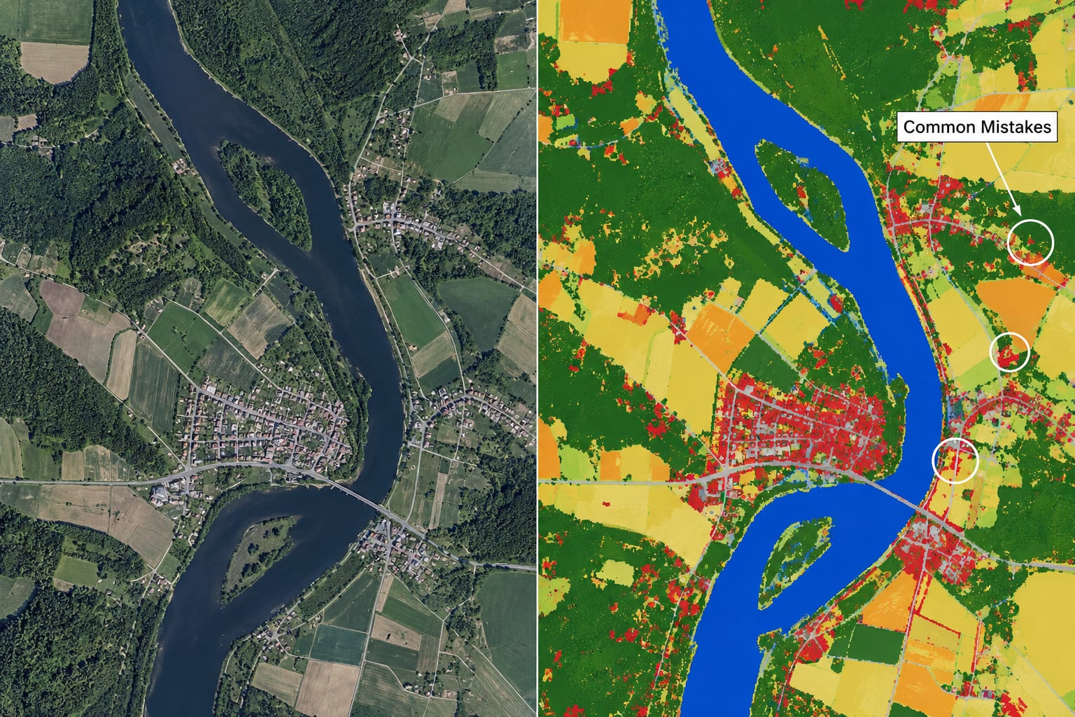
Too few training samples. The most common failure, named as the hardest step by QGIS and remote sensing community users. Under 30 polygons per class, or polygons clustered in one corner, produces a map that only works where you drew. Fix: more samples, spread across the study area, with deliberate variety inside each class.

Confusable classes. Forest against short vegetation, urban against bare soil, cropland against grassland. These pairs overlap physically, so the fix is usually definitional: split the class, drop it, or move to a higher-resolution image. If two classes have nearly identical spectra in every band, no classifier separates them.

Ignoring salt-and-pepper noise. Scattered single pixels inside solid blocks. It comes from mixed pixels along edges and from classes with few samples. Run a modal filter over a 5 by 5 window, but check your accuracy before and after, because filtering always inflates it slightly.

Cloud and shadow contamination. Thin cloud and cloud shadow look like bare soil and water respectively. Mask them before classification, or exclude those pixels from the class they contaminate.

Reporting training accuracy as map accuracy. Validating with your own training data inflates the figure. Hold back an independent set, or use a published dataset as reference.

Wrong projection or pixel alignment. Training polygons that visibly miss their features usually mean a reprojection problem. Confirm every layer shares one coordinate reference system and, for raster training, the same grid alignment.

Following a tutorial written for an older plugin version. QGIS users following SCP v7 walkthroughs hit clipping failures after the preprocessing step on v8 and v9, because the plugin reorganised its band management. Check the version number in the corner of the tutorial against the one in your plugin panel before you start.

Export friction. Reprojection errors when sending GeoTIFF or GeoJSON to Google Earth, and large polygon files that will not render. Clip to the study area before export and use a simplified geometry for web display.

Frequently Asked Questions

Conclusion

Start with the classes, not the software. Write down what each land cover class includes and excludes, check that those distinctions are actually visible in the imagery you plan to use, and collect reference data that is independent of anything you will train on. Once those three are settled, choosing how to classify land cover in remote sensing software becomes a routine: draw samples, run Random Forest or maximum likelihood, filter the speckle, validate with a confusion matrix, and write down your settings so the map can be reproduced.