How to Use a Sample Size Calculator for Research 2026 Guide

A sample size calculator tells you how many participants or records you need before you start, and the honest truth about how to use a sample size calculator for research is that the arithmetic is easy while the assumptions are the hard part. One tool combines your confidence level, the effect or precision you are aiming for, and the variability of your measure, and it does that in five moves: name the analysis, pick the matching calculator, enter defensible assumptions, read the required n, then inflate it for non-response and attrition.

The calculator is the easy part. Almost every bad sample size I have seen in a thesis draft came from an assumption entered in a hurry, not from a calculation error, so this guide spends most of its time on what you put into the fields and how you defend the number afterwards.

Table of Contents

1. 1What You Need
2. 2How to Use a Sample Size Calculator for Research: Step-by-Step
3. 31. Define the research objective and planned analysis
4. 42. Identify the population and eligible participants
5. 53. Choose the statistical inputs
6. 64. Select the correct calculator method
7. 75. Run the calculation and interpret the result
8. 86. Report and justify the sample size
9. 9Common Mistakes
10. 10Frequently Asked Questions
11. 11Is a sample size of 100 enough for quantitative research?
12. 12Why is 30 treated as the minimum sample size?
13. 13What sample size do I need if my population is only 500?
14. 14Should I use a margin of error calculator or a power analysis?
15. 15Can I run a power analysis after collecting my data?
16. 16Conclusion

What You Need

Before you open any calculator, get six things on paper. Each one is a number or a decision that you will have to justify in your methodology section, so write them down as you go.

1. Your study design. Cross-sectional survey, comparison of two groups, pre-test post-test design, repeated measures, cohort, or something with clusters.
2. The planned analysis. The exact statistical test you intend to run: a two-independent-samples t-test, a one-way ANOVA, a chi-square test of independence, a Pearson correlation, or a multiple regression.
3. Population information. The size of the population you are sampling from, and an honest expected response rate.
4. An expected effect or proportion. For estimation work, the population proportion you expect. For hypothesis testing, the standardized effect size you want to be able to detect.
5. A confidence level and power. Conventionally 95% confidence for estimation and 80% power for hypothesis testing, both with alpha set at .05.
6. The right calculator family. A proportion and margin-of-error tool, or a power-based tool such as G*Power or the pwr package in R.

Where do the assumptions come from? The expected proportion and the expected effect size should come from a literature review of comparable studies, or from a pilot, or from your supervisor. Taking 0.5 as the proportion is a deliberately conservative choice rather than an informed one, and that is fine as long as you say so.

Three terms appear constantly, so define them once here. Margin of error is the width of the range around your estimate that you are willing to accept at your stated confidence level. Statistical power is the probability of detecting a real effect of the size you assumed, when one truly exists. Effect size is that real difference expressed in standard deviation units, so that studies with different outcome scales can be compared.

Research methods forums and statistics Q&A sites report the same problem over and over: students arrive with a deadline and a vague question rather than a design. One poster asked for a sample size calculation for a thesis due the next day, and could say only that the previous study had 100 patients. Design first, number second.

How to Use a Sample Size Calculator for Research: Step-by-Step

1. Define the research objective and planned analysis

Start with the sentence you would put in your aim, then map it to a test. If you want to estimate the percentage of staff who intend to leave, you need a proportion calculator. If you want to know whether treatment and control groups differ on a continuous outcome, you need a two-group comparison tool. The test you name here decides the calculator you open next, and that is the first real step in how to use a sample size calculator for research.

The analysis has to be fixed before the calculation, not chosen afterwards. That is what a priori means. If you plan the sample size around one test and then run a different one, the number you justified in your methods no longer applies to the test you actually ran, and a reviewer is entitled to notice.

2. Identify the population and eligible participants

Write down the target population, then the frame you can realistically reach, then your expected response rate. These three numbers determine how many invitations you send, and they also decide whether a finite population correction applies.

The correction matters when your sample is a meaningful fraction of a small, known population. Surveying 400 of the 500 employees in a company does not need the same n as surveying 400 of a city, because there are fewer people left in the population who could have been missed. If you know your population size, enter it into any calculator that offers a population field.

For invitations, the arithmetic is simple. If you need 200 completed responses and expect a 20% response rate, you must contact 200 divided by 0.20, which is 1,000 people. Do this before you start, not after three weeks of disappointing replies.

3. Choose the statistical inputs

This is where most errors happen, because the fields look interchangeable and they are not.

Input fields, what they mean, and the mistake people make

Input	What it means	Typical value	Common mistake
Confidence level	How often the interval would miss the true value across repeated samples	95% (1.96), or 90% (1.645) and 99% (2.576)	Treating it as statistical power
Margin of error	Half-width of the acceptable range around your estimate	Plus or minus 5% for a general survey	Asking for plus or minus 1% without a budget
Expected proportion	The share you expect in the population, used as p(1-p)	0.5 if you have no prior evidence	Guessing 0.2 to look more precise
Alpha	The false positive rate you accept	.05, two-tailed	Switching to one-tailed after seeing direction
Power	Chance of detecting an effect of the assumed size	.80, sometimes .90	Reading .80 as an 80% chance the effect is real
Effect size	Standardized difference you want to detect, such as Cohen’s d of 0.5	0.5 for a medium difference	Entering a p-value in the effect size field
Allocation ratio	Size of group one relative to group two	1.0 for equal groups	Forgetting it when groups are unequal
Population size	Total size of the frame, if known	Leave blank if very large	Omitting it for a small local population

A worked input set for a two-group comparison: standardized mean difference of 0.5, alpha .05 two-tailed, power .80, equal allocation. Power-based calculators return roughly 64 per group, 128 in total, for that combination. Change the assumed effect to 0.3 and the required n rises sharply, which is exactly why the effect size deserves a citation rather than a guess.

4. Select the correct calculator method

Pick the family that matches the analysis from step 1. Anything else and you are answering a question you did not ask.

Which calculator family matches your analysis

Calculator family	Use it when	Key inputs	What it returns
Proportion and margin of error	Estimating a percentage or prevalence	Confidence, margin of error, expected proportion, population	Required completed responses
Mean comparison	Estimating a mean, or comparing two means	Confidence, margin of error or effect size, standard deviation	Required n per group
Two-group comparison	Testing two independent groups or pre-test post-test designs	Alpha, power, Cohen’s d, allocation ratio	n per group
Proportion comparison	Comparing rates between two groups	Alpha, power, expected rates in each group	n per group
Correlation	Testing an association between two continuous measures	Alpha, power, correlation coefficient	Required pairs
ANOVA	Comparing three or more groups	Alpha, power, effect size f, number of groups	Total n across groups
Regression	Predicting an outcome from predictors	Alpha, power, number of predictors, effect size	Total n

Two families exist in practice: margin-of-error calculators, which answer how precise an estimate will be, and power calculators, which answer how likely you are to detect a difference. For a descriptive prevalence survey, use the first. For anything involving a hypothesis test, use the second.

Read the documentation for any calculator you use. Interfaces change; formulas behind them rarely do. For unusual designs such as cluster sampling, multilevel models, or structural equation modelling, the online calculators built for simple tests will not map cleanly, and the forum consensus is to simulate the design in R or use a dedicated package rather than force a match.

5. Run the calculation and interpret the result

Enter the assumptions, read the output, and round up. A calculator returning 384.16 means you need 385, not 384.

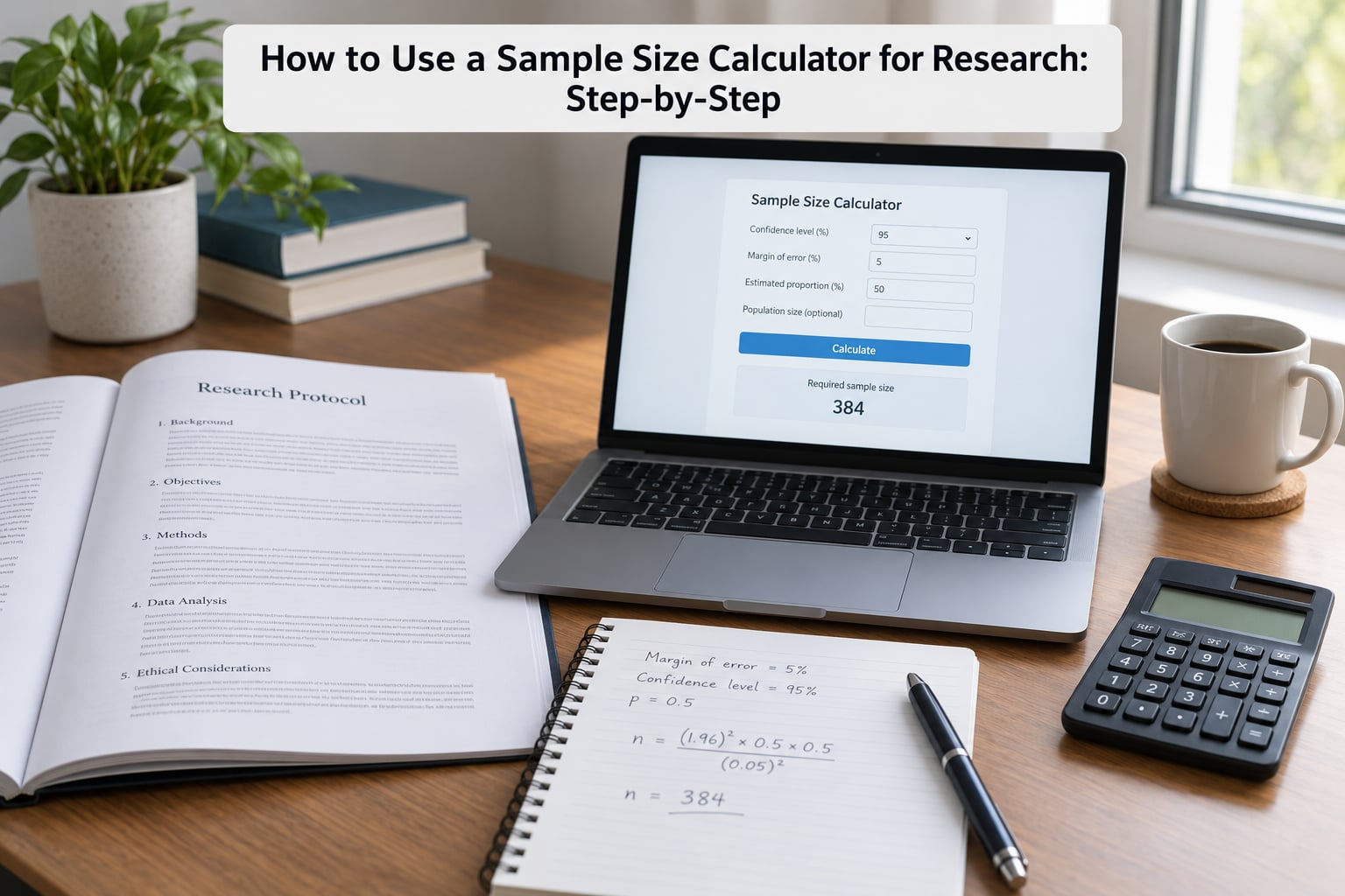
Here is a full example carried through. Question: what proportion of a university population intends to study abroad next year? Calculator: proportion and margin of error. Inputs: 95% confidence, margin of error plus or minus 5%, expected proportion 0.5, population left blank because it exceeds 10,000. Output: n = 384.16, rounded to 385 completed responses.

The plain-text formula behind that result is n = p(1-p)(z / E) squared. Substituting gives n = 0.5 x 0.5 x (1.96 / 0.05) squared, which is 0.25 x 1536.64, or 384.16. Halving the margin of error to plus or minus 2.5% multiplies the requirement by four, to about 1,538. Precision gets expensive fast, and that is a budgeting conversation rather than a statistical one.

Now adjust. At an expected 20% response rate, 385 completions means 385 divided by 0.20, which is 1,925 invitations. With a 15% attrition rate on top of a longitudinal design, inflate again to 385 divided by (0.85 x 0.20), which is about 2,265 contacts. For a clustered design, multiply by a design effect, often between 1.3 and 2.0 depending on cluster size and similarity within clusters, so 385 x 1.5 gives 578. Separate the statistical requirement from the recruitment target and write down both.

One more check before you move on. The 385 figure assumes simple random sampling and full participation. If your respondents self-select, a larger n narrows random error while leaving selection bias untouched.

6. Report and justify the sample size

Write the paragraph while the inputs are still in front of you. A reviewer should be able to reproduce your number from what you wrote.

Sample size was determined by an a priori calculation for estimating a population proportion. The required sample was calculated using a 95% confidence level and a margin of error of plus or minus 5%, with the expected proportion set at 0.5, giving a required sample of 385 completed responses. Anticipating a response rate of 20%, a total of 1,925 potential participants was contacted. Data were analysed in R using the pwr package to verify the calculation.

Name the tool, state every assumption, and say whether the calculation was a priori. Published papers that say sample size was calculated using an online calculator with a 95% confidence level and a stated margin of error are accepted practice; a bare “n = 30 was considered sufficient” is not.

Verify the number yourself rather than trusting the page. Recompute the proportion example by hand as shown above, then rerun it in R with pwr or a package such as samplesize, or open the same analysis in G*Power and confirm it lands within a person or two. Different tools round differently, and a mismatch of one or two is normal; a mismatch of forty means an assumption differs and you need to know which one.

That verification habit answers the most common forum complaint about these tools. People want the formula so they can check a calculator rather than take it on trust.

Common Mistakes

1. Using a generic calculator for a design it does not model. Correction: match the tool to your planned test. A proportion calculator cannot tell you the n for a two-group t-test.
2. Entering a p-value into an effect size field. Correction: an effect size is a standardized magnitude such as Cohen’s d of 0.5, not a probability.
3. Ignoring non-response. Correction: divide the required n by your expected response rate and round up. The 385 figure is completions, not invitations.
4. Treating power as a guarantee. Correction: 80% power means an 80% chance of detecting an effect of the assumed size in a study where that effect genuinely exists. It says nothing about whether the effect exists.
5. Changing assumptions after seeing the results. Correction: keep the a priori calculation in the record and report it as planned. Running a post hoc power analysis on observed data is circular, because the calculation is built from the very result it is meant to explain.
6. Failing to match the sample to the analysis. Correction: state the test in your methods and confirm the calculator used that same test.
7. Grabbing a round number from folklore. Correction: 30 is not a minimum, and the rule of ten participants per variable is a screening heuristic for stable regression coefficients, not a justification a reviewer will accept. A community thread with a thesis due the next day turned on exactly this kind of borrowed number.

Before you submit, run this checklist: the planned analysis is named; the calculator family matches it; the confidence level and alpha are stated; the effect size or proportion has a source; the population size is entered if it is small; the output was rounded up; response rate and attrition were applied; the design effect was applied if sampling is clustered; and the tool used is named in the methods.

Frequently Asked Questions

Conclusion

Start by writing one sentence: the analysis you intend to run and the assumption it turns on. Pull the expected effect or proportion from a cited source, run the matching calculator, round up, then inflate for response rate and attrition before you write the methods paragraph. That sequence is the whole of how to use a sample size calculator for research, and it is unchanged as of 2026 even though every calculator interface you use will eventually be redesigned.