Slope analysis turns a digital elevation model into a raster where every cell holds how steep the ground is at that point, in degrees or percent grade. Learning how to use DEM data for slope analysis takes about 30 minutes once you know the workflow, and the whole thing runs in QGIS, ArcGIS Pro or a GDAL command. The hard part is not the tool. It is setting the Z factor correctly and picking a DEM whose resolution matches the decision you are trying to make.
Walk through the process below and you will end up with a classified slope map, a per-feature average slope table if you need one, and a validation checklist you can defend in front of a reviewer.
Table of Contents
- 1What You Need for DEM Slope Analysis
- 2The DEM itself
- 3Software
- 4A projected coordinate system
- 5A slope unit decision
- 6Step-by-Step: How to Use DEM Data for Slope Analysis
- 7Step 1: Prepare and Inspect the DEM
- 8Step 2: Choose the Correct Spatial Resolution
- 9Step 3: Calculate the Slope Raster from DEM Data
- 10Step 4: Select Degrees or Percent Grade
- 11Step 5: Classify and Interpret the Results
- 12Step 6: Validate and Export the Slope Map
- 13Common Mistakes and How to Fix Them
- 14Frequently Asked Questions
- 15What is the best software for DEM slope analysis?
- 16Should slope be calculated in degrees or percent?
- 17What DEM resolution is suitable for slope analysis?
- 18Why does my slope map show zero values in areas that are not flat?
- 19Can DEM data calculate slope in areas with missing elevation values?
- 20What is the difference between slope and aspect in GIS?
- 21Conclusion
What You Need for DEM Slope Analysis
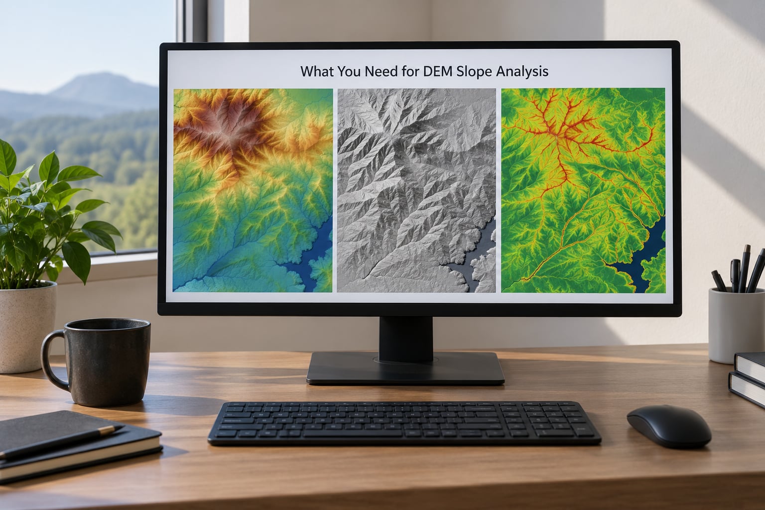
You need four things: a DEM, a GIS that can run terrain derivatives, a projected coordinate system in metres, and a decision about which slope unit you are reporting in. That is the whole list.
The DEM itself
For most regional work, a public DEM will do: SRTM at roughly 30 m, or Copernicus GLO-30 at about 30 m, both downloadable from USGS and ESA sources. For site-scale work you want a LiDAR-derived DTM at 1 to 2 m from your local survey or open data portal.
Check the metadata before anything else, because the same dataset can behave very differently depending on whether you have a bare-earth DTM or a DSM that still includes tree canopy and rooftops. A DSM produces false steep edges around every building and every stand of trees, and those artefacts will dominate your slope output at fine resolution.
Software
QGIS and ArcGIS Pro both ship a slope tool out of the box. GDAL, the library underneath most open-source GIS, has gdaldem slope for anyone who prefers a terminal or wants to batch-process hundreds of tiles. Google Earth Engine can do it too, but through a different API.
A projected coordinate system
Slope is a ratio of rise to run, and run only makes sense in linear ground units. If your DEM is in geographic coordinates such as EPSG:4326, one degree of longitude is not the same distance as one degree of latitude, so you must reproject to a projected CRS with metre units before you calculate anything. A local UTM zone is the usual choice.
A slope unit decision
Decide now whether the deliverable is in degrees or percent grade. Degrees describe terrain angle for mapping and hazard screening. Percent grade is what road designers, drainage plans and accessibility rules use. Changing later means reinterpreting every threshold you picked, so settle it before the calculation, not after.
Step-by-Step: How to Use DEM Data for Slope Analysis

The full workflow has six stages. Inspect the DEM, match its resolution to your decision, run the slope tool, pick the output unit, classify the values into bands, then validate and export. Every stage below says what to do and how to tell it worked.
- Load the DEM and check its CRS, cell size, elevation range and voids.
- Reproject and resample to a projected CRS at a cell size your decision can actually resolve.
- Run the slope tool with a correct Z factor to produce a new raster.
- Choose degrees or percent grade as the output unit.
- Classify the raster into usable bands, then polygonize or run zonal statistics.
- Validate the output against known terrain, then export with a legend and metadata.
A good slope raster has a value in every valid cell, a sensible histogram, and steep pixels exactly where the land is steep. If your output is uniform black, uniform white, or striped with gaps, stop and read the mistakes section rather than pushing the file into a report.
Step 1: Prepare and Inspect the DEM
Load the raster into QGIS with Layer and then Add Raster Layer, or in ArcGIS Pro use Map and then Add Data. Before touching any tool, open Layer Properties and read four fields.
First, the coordinate reference system. If it is geographic rather than projected, that is your first fix. Second, the source cell size, shown under Source in the properties panel. Third, the elevation range, found by opening the Layer Properties histogram or by running raster statistics. A range of zero to a few hundred metres is normal; a range near zero usually means the file failed to load properly.
Fourth, the voids. Zoom to the raster edges and look for black or transparent blocks, especially if your data came from SRTM, which is assembled from scene strips and can leave gaps where scenes do not overlap. Those voids become NoData in the slope output and will not show up in the histogram unless you exclude NoData from the statistics.
Also decide whether you are holding a DTM or a DSM. Bare earth is what you want for almost every slope decision. At 30 m resolution the difference barely matters. At 1 to 2 m from LiDAR it matters enormously.
Step 2: Choose the Correct Spatial Resolution
Resolution sets the smallest landform your slope raster can possibly show, and it changes the numbers. Coarsening cells smooths detail, which pushes mean and maximum slope downward. Comparing slope values derived from two different resolution DEMs is not a valid comparison, which is the single most overlooked trap in this kind of work.
| Decision you are making | Landform scale | Suggested cell size | Typical source |
|---|---|---|---|
| Continental hazard screening, regional suitability | 10 km and larger | 90 to 1000 m | ASTER GDEM, SRTM at coarse resampling |
| Catchment planning, agricultural plot productivity | 100 m to 2 km | 10 to 30 m | SRTM, Copernicus GLO-30 |
| Road alignment, parcel-level development siting | 5 to 50 m | 2 to 5 m | Copernicus GLO-30 resampled, regional LiDAR |
| Site engineering, slope stability screening | Under 5 m | 0.5 to 1 m | LiDAR-derived bare-earth DTM |
Resample only when you must, and choose the method deliberately. Bilinear or average aggregation is right when you are smoothing an existing DEM down. Nearest neighbour is right when your cell values are classes rather than continuous measurements. Running a slope tool on a nearest-neighbour resampled DEM produces blocky stair-stepped results that look wrong because the elevation surface itself is now stepped.
Step 3: Calculate the Slope Raster from DEM Data
The slope tool reads the elevation difference between each cell and its eight neighbours, converts that rise over run into an angle, and writes one slope value per cell into a new raster. QGIS, ArcGIS Pro and GDAL all do exactly this, and their settings differ only in wording.
| Workflow step | QGIS 3.x | ArcGIS Pro | GDAL command line |
|---|---|---|---|
| Find the tool | Processing Toolbox, then Raster terrain analysis, then Slope | Analysis and then Raster surface, then Slope | gdaldem slope |
| Input | Elevation layer | Input raster | Input DEM filename |
| Z factor | Scale and Z factor parameter, set to 1 for metre-based projected CRS | Z factor, set to 1 for metre-based projected CRS | -z 1 |
| Units | Output as Degrees or as Horizontal Percentage | Output measure, Degrees or Percent | -p for percent, omit for degrees |
| Output | Output raster path, GeoTIFF | Output raster, GeoTIFF to a folder | Output GeoTIFF filename |
In QGIS, the equivalent command line reads roughly gdaldem slope input_dem.tif slope.tif -p -z 1 -of GTiff. In ArcGIS Pro the tool lives under Analysis, then Raster surface, then Slope, where you set the input raster, the output measure and the cell size.
You can tell it worked by checking three things. The output range should top out below 90 degrees, because slopes beyond 90 degrees are not physically possible on a land surface and usually indicate bad input. The histogram should be right-skewed, with most cells at low values. And the steepest pixels should sit along valley walls, escarpments and cut banks, which you can confirm by putting a hillshade underneath as a semi-transparent layer.
One community answer worth knowing: on Reddit r/QGIS the practical path beginners get told repeatedly is hillshade first for orientation, then the GDAL slope algorithm from the Processing Toolbox. Both produce a usable result, so pick whichever you can repeat reliably across every tile in your project.
Step 4: Select Degrees or Percent Grade
Degrees and percent grade describe the same slope in different maths. Degrees is the angle of the incline from horizontal. Percent grade is that rise as a ratio to horizontal distance, so 100 percent is 45 degrees and 5 percent is about 2.86 degrees.
Use degrees for terrain description, hazard screening and most thematic maps. Use percent grade whenever a limit is written as a ratio, because road grades, drainage rules and accessibility standards are all phrased that way.
| Percent grade | Degrees | Typical use |
|---|---|---|
| 2% | 1.15 | Drainage falls on paved surfaces |
| 5% | 2.86 | Accessibility ramp maximum running slope |
| 6 to 8% | 3.43 to 4.57 | Main road and highway grade limits |
| 10% | 5.71 | Residential street grade |
| 12 to 15% | 6.84 to 8.53 | Mountainous road stretches |
| 25% | 14.04 | Rough upper limit for construction without major earthworks |
| 45% | 24.23 | Very steep, erosion and mass movement likely |
Converting between them is straightforward: percent equals the tangent of the degree angle, multiplied by 100. The reverse uses the arctangent. Set the unit in the slope tool itself rather than converting the raster afterwards, so the Z factor and units stay consistent with the source data.
Step 5: Classify and Interpret the Results
A continuous slope raster is hard to read on a map and hard to threshold in a rule. Reclassify it into named bands first. In QGIS use Raster and then Reclassify by table, or Process and then Raster calculator; in ArcGIS Pro use the Reclassify tool on the Classification menu.
Pick break values that match the decision rather than round numbers. A typical suitability classification looks like this: 0 to 5 percent as flat, 5 to 15 percent as gentle, 15 to 30 percent as moderate, 30 to 45 percent as steep, and above 45 percent as very steep. For a road or accessibility study, tighten those breaks around the regulatory limits instead, so the classes straddle the thresholds that actually matter.
Then check the raster statistics before you trust the picture. Look at mean, standard deviation, minimum and maximum. A standard deviation near zero means your slope surface has almost no variation, which usually points back to a resolution or Z factor problem rather than genuinely flat terrain.
Two cleanup steps make the output much more usable. Run Sieve to drop single-cell speckle, the small isolated steep pixels that come from noise or from DSM artefacts around buildings. Then run Polygonize to convert the classified raster into vector polygons, one polygon per class, which is what you need for area summaries, map production or a table you can join to parcel data.
If you already have polygons and you want a single number for each one, zonal statistics answers that directly. The most common practitioner question on GIS StackExchange is exactly this: someone downloads a NASA DEM for a study area, converts it to slope, and then wants the slope of each farm polygon rather than a raster. Use Zonal Statistics as Table in QGIS, or Zonal Statistics in ArcGIS Pro, with the slope raster as the value field and your polygons as the zone data. Add mean, maximum and minimum as statistics so you can see whether a parcel is uniformly gentle or sharply broken.
Step 6: Validate and Export the Slope Map
Validation is what separates a slope map you can defend from one you cannot. Run these checks before exporting anything.
- Confirm the maximum value is under 90 degrees and the minimum is zero or above.
- Check that the CRS is projected and in metres, and that the Z factor you entered matches those units.
- Compare a handful of known slopes. Sample a steep riverbank, a flat valley floor and a known road cut, and check that the values make sense.
- Overlay a hillshade at 40 to 50 percent transparency to confirm the steep zones align with visible relief.
- Confirm that NoData gaps are intentional rather than the leftovers of scene seams.
- Record the DEM source, version, date, vertical datum and Z factor in the map metadata.
Export the slope raster as GeoTIFF so it stays georeferenced, and export your map layout as PDF with a legend, units and a north arrow. Keep the unclassified raster alongside the classified version, because someone will always ask for the raw values later.
One honest limit: slope derived from a DEM is a screening proxy. It describes terrain gradient, not shear strength, pore pressure or factor of safety. Landslide susceptibility work needs geotechnical inputs on top of the slope layer, and no amount of DEM resolution replaces them.
Common Mistakes and How to Fix Them
Most of the time, how to use DEM data for slope analysis goes wrong at the setup stage rather than inside the slope tool itself. Almost every wrong slope map traces back to one of a handful of causes, and the table below maps what you see to what is actually wrong and what to change.
| Symptom | Likely cause | Fix |
|---|---|---|
| Everything looks flat, values near zero | DEM is in geographic degrees, so Z factor 1 treats one degree as one unit of rise | Reproject to a projected CRS in metres, then rerun with Z factor 1 |
| Slope looks far too steep | Z factor left at 1 while the CRS is geographic, or vertical units are feet | Set Z factor to 1 for metre units, about 3.28084 for feet |
| Entire raster is uniform black or empty | NoData across the whole extent, or an elevation band was not recognised | Check the histogram with NoData excluded, then fill voids or clip to valid extent |
| Striped gaps across the output | SRTM scene seams carried through as NoData | Mosaic tiles before analysis, or use a different DEM source such as Copernicus GLO-30 |
| Spiky isolated cells everywhere | Single-cell noise or DSM artefacts from canopy and buildings | Run Sieve to remove speckle, or switch to a bare-earth DTM |
| Slope values inconsistent between two study areas | The two DEMs have different cell sizes or vertical datums | Resample both to the same resolution and common vertical datum before comparing |
| Map looks blocky or stepped | Nearest-neighbour resampling applied to continuous elevation values | Resample with bilinear or average aggregation instead |
| Confusing steepness with direction | Slope and aspect mixed up in the output legend | Slope gives steepness in degrees or percent, aspect gives compass direction |
| Zeros in areas that are clearly not flat | Flattened voids filled with a constant elevation, or a zonal statistic averaging over filled cells | Restore true elevation values, or report mean slope excluding NoData cells |
As a general habit, check the histogram before you style the map. Most of these problems are obvious in the distribution of values and invisible in the colour ramp.
Frequently Asked Questions
What is the best software for DEM slope analysis?
QGIS is the strongest default because it is free, its Processing Toolbox includes both the GDAL slope algorithm and a native raster slope tool, and it runs on Windows, macOS and Linux. ArcGIS Pro does the same job with a licence and better integration with Esri geodatabases. GDAL command line suits batch work across many tiles. All three produce the same slope values from the same DEM if the Z factor and units match, so choose on cost, licensing and how many tiles you need to process.
Should slope be calculated in degrees or percent?
Use degrees for terrain description, hazard screening and thematic maps, because that is how slope is normally reported in the literature. Use percent grade when your decision is written as a ratio, such as road grade limits, drainage falls or accessibility ramp rules. Set the unit inside the slope tool rather than converting the raster afterwards. A 10 percent grade is 5.71 degrees, and 100 percent is exactly 45 degrees.
What DEM resolution is suitable for slope analysis?
Match the cell size to the smallest landform your decision depends on. Around 30 m suits catchment and agricultural work, 2 to 5 m suits road alignment and parcel siting, and 0.5 to 1 m suits site engineering. Resolution changes the computed value, so mean and maximum slope fall as cells coarsen, and slope from two different resolution DEMs should never be compared directly without resampling first.
Why does my slope map show zero values in areas that are not flat?
Zero usually means the tool had no valid elevation to work from. Common causes are NoData gaps at the raster edges or SRTM scene seams, voids filled with a constant value, or a polygon whose cells were all excluded during a zonal statistic. Check the histogram with NoData excluded, zoom to the zero cluster at full raster resolution, and inspect the source DEM at that location. Flat terrain that genuinely measures zero is rare in real elevation data.
Can DEM data calculate slope in areas with missing elevation values?
Not from the missing area itself. A slope cell needs valid elevations in its neighbourhood, so cells surrounded by NoData come out as NoData rather than a slope value. Most DEM sources ship free gap-filled products, and merging tiles before analysis removes the striped gaps that scene boundaries leave behind. Where no public DEM covers your area, you can build one from contour lines or surveyed elevation points with a TIN interpolation, then run the same slope tool on the result.
What is the difference between slope and aspect in GIS?
Slope measures how steep the ground is, expressed in degrees or percent grade, with zero meaning flat. Aspect measures which direction the slope faces, expressed as a compass bearing from zero to 360 degrees. They are separate derivatives of the same DEM and answer different questions. Slope decides whether a site is buildable and how water will shed; aspect decides solar exposure, which matters for vegetation, snow melt and building orientation.
Conclusion
Start by opening your DEM’s properties and checking two things: whether the CRS is projected in metres, and whether you hold a DTM or a DSM. Everything downstream depends on those two answers.
Once the slope raster exists, classify it against thresholds you can justify, overlay a hillshade to check the result against the real terrain, and record your DEM source and Z factor in the metadata. If you need a single number per parcel rather than a map, run zonal statistics on the polygons next. That is the step most projects are missing when a client asks why they have a raster but no answer per field.