How to Interpolate Point Data into a Surface: GIS Guide 2026

To interpolate point data into a surface, you estimate the values you never measured by weighting the measurements you did take, then write those estimates to every cell of an output raster. The workflow is the same in QGIS, ArcGIS Pro, R and Python: inspect the points, pick a method that matches how the variable behaves in space, set the output grid, run it, and check the result against held-out samples. Give it 30 to 60 minutes on a small dataset once you have done it a couple of times.

Spatial interpolation rests on one idea, usually credited to Tobler’s first law of geography: everything is related to everything else, but near things relate more strongly than far things. That is the entire justification for drawing a continuous surface across the gaps in your samples, and it is also why the geometry of your points matters as much as your choice of algorithm. Updated for October 2026.

Table of Contents

1. 1What You Need
2. 2Step-by-Step
3. 31. Inspect and Prepare the Point Data
4. 42. Choose an Interpolation Method
5. 53. Set the Output Grid and Parameters
6. 64. Run the Interpolation and Inspect the Raster
7. 75. Validate and Document the Surface
8. 8Common Mistakes
9. 9Quick Tips for a Reliable Interpolation Workflow
10. 10Frequently Asked Questions
11. 11What is the difference between interpolation and extrapolation?
12. 12Which GIS software can interpolate point data into a surface?
13. 13Is inverse distance weighting better than kriging?
14. 14How do I choose the cell size for an interpolated raster?
15. 15Can an interpolation map show uncertainty?
16. 16Why do my interpolated values differ from the original point values?
17. 17Conclusion

What You Need

You need a point layer, a value field, and a decision about what the surface is for. The rest is software and care.

• A point layer with coordinates. Each feature needs an X and Y in the same spatial reference for every other feature. GPS coordinates stored in decimal degrees are fine as long as you project them before you interpolate.
• A numeric field to interpolate. Elevation, rainfall totals, contaminant parts per million, soil pH. Categorical fields cannot be interpolated with these methods.
• Enough sample coverage. Aim for at least 10 points, and treat anything under 30 as provisional. In practice you want points spread across the whole study area, not a tidy cluster along one road.
• A projected spatial reference. Interpolation measures distance, and distance measured in degrees is wrong. Use a projected CRS in metres for your region, such as a national coordinate system or an equal-area projection.
• The study-area boundary. A polygon or mask so you do not end up with cells floating in space where no sample ever existed.
• A GIS package. QGIS or ArcGIS Pro for a visual workflow, or R and Python if you want the whole thing scripted and reproducible.

The one people skip is the last decision. A surface for pretty contour lines has different requirements than a surface feeding a flood model or a kriging-based risk map, and the downstream use should drive the method, not the other way round.

Step-by-Step

1. Inspect and Prepare the Point Data

Open the layer and look at the fields before you touch an interpolation dialog. Check that your value field is numeric rather than stored as text, which is the single most common reason a tool refuses to run or silently returns blanks.

Then remove the obvious problems. Look for duplicate coordinates, often the same station sampled twice with slightly different values, and null or flagged values such as a recorded 9999 placeholder for missing data. Drop invalid geometry and any point that sits far outside the study boundary, since those will drag a local surface badly.

Plot the points and look at their distribution. A tight cluster in one corner with nothing else is not a surface, it is a guess. Note the spacing and any linear gaps: if your samples follow roads, a road, ridge or river is a barrier, and interpolation will happily smear values across it unless you tell the tool not to.

Confirm the coordinate reference system in the layer properties. If any point has been entered in a different system, reproject the whole layer to your target projected CRS before anything else, and keep the raw file untouched. Version control for spatial data is not a joke; I have lost an afternoon to an overwritten attribute table that only existed in a shapefile backup from earlier that year.

Finally, decide whether values need transforming. Pollution and concentration data are usually strongly right-skewed, and interpolating a log or normal-score transform and back-transforming afterwards usually produces a far better surface than interpolating the raw values.

2. Choose an Interpolation Method

Choose based on three things: how densely and evenly your points are spread, whether the variable has a known trend across the area, and whether you need an uncertainty surface. There is no universal best method, which is why people get stuck.

Inverse distance weighting (IDW) is the quick, defensible default. Each nearby point gets a weight of 1 divided by its distance to a power p, and the prediction is the weighted average. A surface passes exactly through every sample point. It needs no variogram, it is fast, and it is easy to explain in a methods section. Power p between 1 and 5 is the usual range; 2 is the default and a reasonable start.

A quick worked sense of it: if you have two samples, one at 1,000 m with a value of 12 and one at 3,000 m with a value of 20, and you predict at 2,000 m with p = 1, the weights are 1/1000 and 1/3000, giving (0.001 × 12 + 0.000333 × 20) / 0.001333 = 14. In a spreadsheet that is one line of arithmetic; the raster version does it for every cell.

Natural neighbour interpolation (also called natural neighbour IDW or NatNad, or Thiessen polygons in its simplest form) builds a Voronoi diagram and moves values between neighbours only as the estimated point crosses their shared boundary. It is exact, non-iterative, and handles clumped or irregular sample distributions better than IDW because it is not thrown off by the distance between clusters. This is a common first pass and a good sanity check before kriging.

Spline interpolation (regularised or tension) fits a smooth rubber sheet through every point. It gives the smoothest and most visually attractive surface and is popular for elevation and rainfall, but it overshoots at the edges and can invent ridges and hollows between widely spaced samples. Regularised spline minimises curvature; tension spline minimises overshoot and behaves better with clustered data. Use tension if your points are uneven.

Kriging is the geostatistical option, and the one to reach for when the result has to go in a report or feed a model that needs error. It uses a semivariogram, a function describing how disagreement between nearby samples grows with distance, to weight points and to estimate how much the prediction might be wrong. Ordinary kriging assumes no overall trend; universal kriging fits and removes a trend first. Kriging gives you a prediction standard error surface, and nothing else in this list does.

Trend surface regression fits a smooth polynomial to the coordinates and ignores local detail. It is appropriate when the pattern really is broad and gradual, such as a regional gradient, and wrong for anything with local structure.

Method	Passes through sample points	Sample distribution	Barrier support	Uncertainty output	Best used for
Thiessen polygons	Yes	Any, even clumped	Yes	No	Closest-station maps, first pass
Inverse distance weighting	Yes	Dense and even	Yes	No	General-purpose, fast previews
Natural neighbour	Yes	Clumped or irregular	Limited	No	Coverage, distribution maps
Spline	Yes	Fairly even	Via tension parameter	No	Elevation, rainfall, smooth fields
Ordinary kriging	Yes	Even, with spatial autocorrelation	Yes	Yes	Published surfaces, risk modelling
Universal kriging	Yes	Even, with a clear trend	Yes	Yes	Data with a regional gradient
Trend surface	No	Any	No	Yes	Broad smooth patterns only

For most assignments and most datasets, the honest sequence is: run Thiessen polygons to check coverage, run IDW to get a baseline surface, then run kriging with a modelled variogram and compare the three by cross-validation. Whichever wins on error, with a caveat you can defend, is your answer.

One more decision that gets skipped. If there is a real discontinuity in the data, a fault line, a cliff, a deep river channel or a sharp land-use boundary, use it. ArcGIS Pro’s IDW, spline and kriging tools all accept barrier or breakline features; QGIS exposes them differently depending on the algorithm and provider. Skipping this step is why people get a surface with a river smoothly climbing a 30 m bank.

3. Set the Output Grid and Parameters

The output grid is where most beginners go wrong. You set the extent of the raster, its cell size, how many neighbours each prediction may use, and where the result is written.

Set the extent to the study-area boundary or to a slightly padded hull around your points, then clip or mask afterwards. Leave it as the default full bounding box and you will produce cells far outside your data that look like surface but are extrapolation.

For cell size, take the median spacing between your sample points, or about half of the smallest meaningful feature you want to resolve. Do not set a 1 m grid from 300 m sample spacing. A finer grid interpolates the same information into more cells; it does not add information, it just inflates the file and invites false confidence in the output. A useful rule is that your cell size should be no smaller than half the typical distance between samples.

For IDW, the power parameter and the number of points or search radius decide the shape of the surface. Twelve nearest neighbours is a common starting point. Increase it for smoother results, decrease it where you need local detail and have dense samples.

For kriging, the semivariogram model and the neighbourhood matter most. Model the experimental semivariogram first, check that the nugget, sill and range make sense, then use ordinary kriging unless a trend is clearly present. Keep the same number of neighbours across methods you are comparing, otherwise the comparison is meaningless.

4. Run the Interpolation and Inspect the Raster

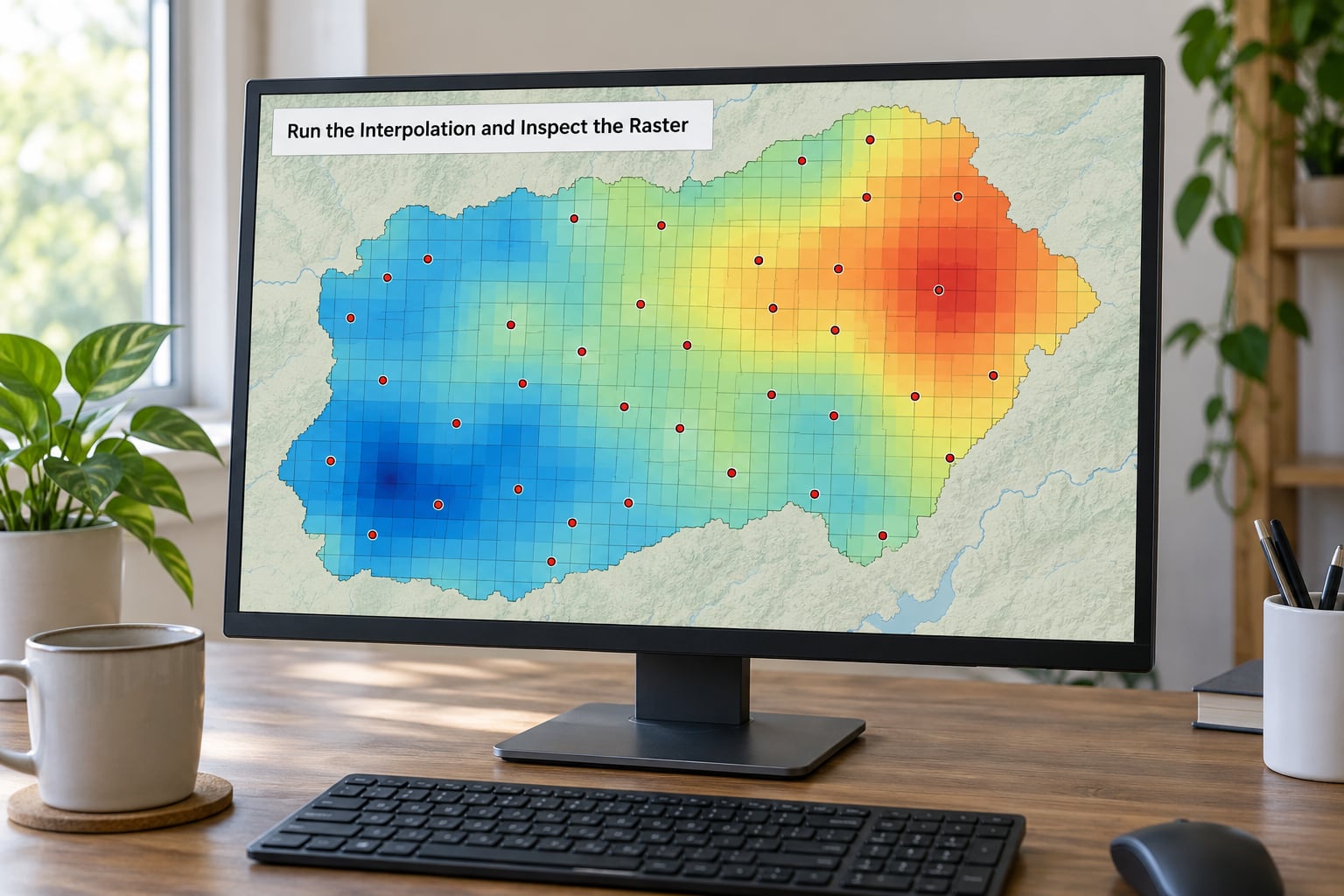
In QGIS 3.x, open Processing and search for IDW Interpolation. Choose your point layer, the value field, the output cell size and extent, the power parameter and the number of neighbours, then run it and load the result. Kriging is in the same toolbox as Ordinary Kriging and Empirical Bayesian Kriging; Natural neighbour sits alongside them. Empirical Bayesian Kriging automates the variogram modelling, which is convenient, though analysts on the Esri forums and GIS Stack Exchange regularly point out that it gives you less control than fitting the model yourself.

In ArcGIS Pro, use the geostatistical tools in the Spatial Analyst or Geostatistical Analyst extension: IDW, Natural Neighbor, Spline, Ordinary Kriging. Each writes a prediction surface, and the kriging variants can also output a standard error surface. The older Interpolate Points tool is a general-purpose predictor for values at specific locations rather than a full raster workflow.

In Python, scipy.interpolate.griddata gives you linear and nearest-neighbour interpolation in a couple of lines, PyKrige covers IDW, ordinary kriging, universal kriging and regression kriging with proper variogram models, and scikit-gstat offers exploratory variogram analysis and variogram modelling. In R, the automap package automates kriging, gstat gives you full control including variogram fitting and cross-validation, and fields is well suited to larger grids.

import numpy as np
from pykrige.ok import OrdinaryKriging

ok = OrdinaryKriging(
    x, y, values, variogram_model="linear",
    variogram_parameters={"slope": 1.0, "intercept": 1.0}
)
predictions, sigma = ok.execute("grid", grid_x, grid_y)

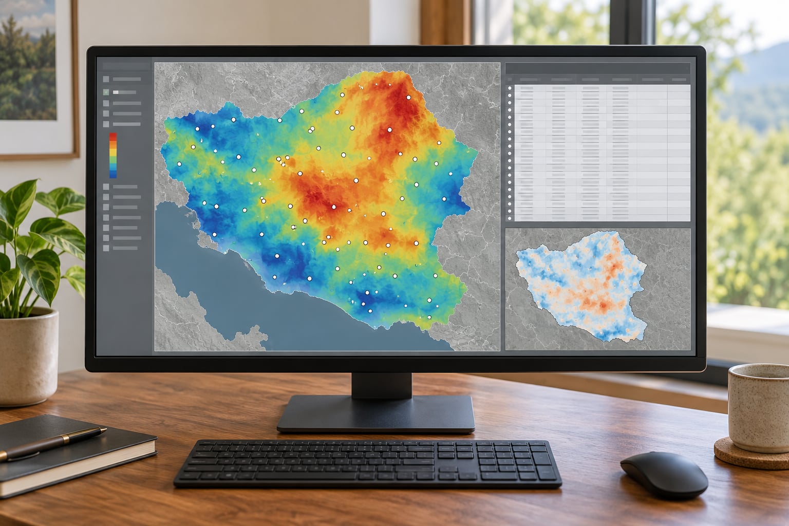
Inspect the output before you believe any of it. Look for NoData holes inside the study area, which usually means too few points fall inside the search neighbourhood. Look for concentric rings around each sample, the classic IDW bullseye, and for spikes or pits that no sample supports. Check the edges: values pressed up against the extent boundary are extrapolation, not interpolation.

Overlay the original points on the surface. Every exact interpolator should pass through each sample point, so any point sitting visibly off the surface means the point layer and the raster disagree, most often because one was reprojected and the other was not. Then check the value range. If your samples run from 4 to 19 and the raster spans 2 to 31, spline or a low power value has overshot, and you should either switch methods or transform the data.

Large point sets need planning. Datasets above roughly 150,000 points are a well-known performance cliff in desktop GIS, with tools appearing to hang and users reporting crashes. Aggregate to a coarser grid, thin the samples with a spatial subset, or move to the code libraries, which handle far more points when you avoid building an enormous output grid in memory.

5. Validate and Document the Surface

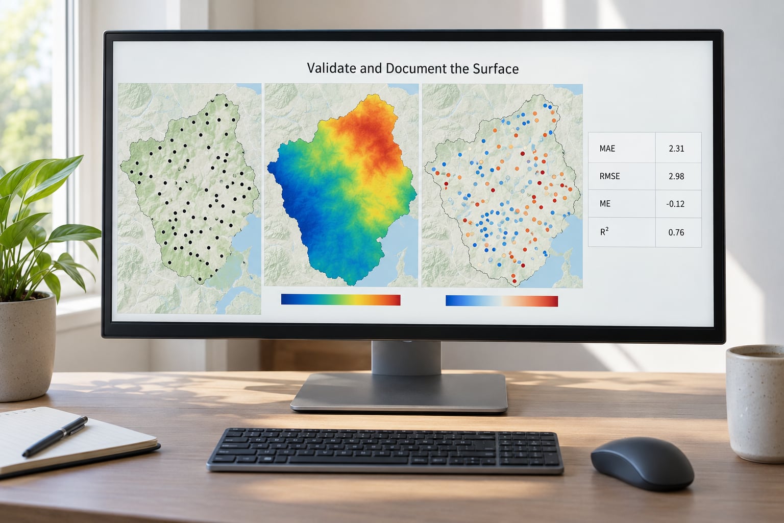
Validation means testing the surface against data that did not build it. The standard approach is cross-validation: remove one point, interpolate the remaining set, predict the removed point, repeat for every point, and summarise the errors. Report root mean square error and mean absolute error, and report them for each method you tried rather than only the winner.

Do not validate with the points you interpolated from. A surface that passes exactly through every input point will score near-perfectly and tell you nothing. GIS Stack Exchange threads on interpolation accuracy keep running into the same confusion.

Then inspect the residuals rather than only the summary number. Plot observed minus predicted against the predicted value and against location. A wedge or funnel in a scatter of observed against predicted is the classic sign that you should have fitted a trend, so universal kriging or a transform is worth trying.

If your method produces one, keep the prediction standard error surface and publish it next to the predictions. Reviewers and decision-makers increasingly expect an uncertainty layer, and kriging gives it to you for free.

Write down what you did so someone else can repeat it: the CRS, the cell size, the method, every parameter value, the variogram model and its fitted parameters, the input data version, the cross-validation error statistics and the software and version. That paragraph takes five minutes and saves an entire argument later.

Common Mistakes

These six account for most broken interpolation results I have seen, and most appear again and again on GIS Stack Exchange, r/gis and r/QGIS.

Interpolating in a geographic coordinate system. Weights computed from degrees give nonsense results away from the equator. Fix: project to a projected CRS in metres before interpolating, and record it.

Ignoring clustered or uneven samples. Twenty points along one road produce a confident surface across a whole county. Fix: check the distribution map before you run anything, and if coverage is genuinely poor, add samples or narrow the study area to what you can defend.

Using a smooth method across a barrier. Spline and IDW will bridge a cliff, a fault or a channel unless you supply barrier features. Fix: pass your breaklines to the tool, or accept that your surface is only valid within homogeneous zones.

Choosing an excessively fine grid. A 1 m raster from 500 m samples is a picture of the data, not extra precision. Fix: set the cell size to the median sample spacing or coarser, then aggregate for display if you want a finer picture.

Extrapolating past your samples. Cells beyond the outermost points are model output driven by assumptions, not measurements. This is also the most common cause of “my interpolation does not cover the whole study area”, where the tool either leaves NoData outside the search radius or invents values. Fix: mask the raster to a boundary and add sample points near the edges if you genuinely need coverage there.

Validating with the input points. Exact interpolators reproduce their inputs by definition, so the error looks perfect and means nothing. Fix: withhold points, or use cross-validation.

Quick Tips for a Reliable Interpolation Workflow

• Run more than one defensible method and let cross-validation pick, rather than letting habit pick.
• Keep the raw point file untouched; reproject and clean into a new layer so you can start over.
• Transform skewed data such as concentrations before interpolating, and say so in the write-up.
• Report the spatial reference, cell size, method and parameters. It takes one sentence and removes an entire class of argument.
• Mask the raster to the valid study area so nobody reads the extrapolation as observation.
• Treat the surface as an estimate. Somewhere between samples you are describing a model’s opinion, not a measurement.
• Decide early whether you need uncertainty, because that rules out IDW and spline and points you toward kriging.

Frequently Asked Questions

Conclusion

Start by inspecting your point layer, since the distribution and spatial reference decide what is possible. Choose a method that matches the variable: IDW for a defensible general default, natural neighbour for clumped samples, tension spline for smooth fields, kriging when you need uncertainty.

Then build one coarse test surface, validate it against held-out points with cross-validation, compare it against a second method, and record the CRS, cell size and every parameter you used. Whatever wins on error, ship with its uncertainty layer and a clear statement of where interpolation stops and extrapolation begins.