How to Run Spatial Autocorrelation and Interpret Morans I 2026

To run spatial autocorrelation and interpret Moran’s I, you need three things in the right order: a clean georeferenced dataset, a spatial weights matrix you can defend in writing, and a permutation test that tells you whether the observed value is unusual. The whole procedure takes about 20 minutes once your data are in shape.

Moran’s I, published by P.A.S. Moran in 1950, compares every value with a weighted average of its neighbours, then summarizes that comparison as one number. Values above the expectation of -1/(n-1) point to clustering, values below it point to dispersion, and a non-significant result is only a statement about the scale you chose.

I have watched people get this wrong for years, and it is almost never the mathematics. It is the weights matrix, or testing the raw variable when they meant to test residuals. Let’s walk the whole workflow.

Table of Contents

1. 1What You Need
2. 2Step-by-Step
3. 31. Inspect and prepare the spatial data
4. 42. Build and justify the spatial weights matrix
5. 53. Run Moran’s I in GeoDa
6. 64. Run Global Moran’s I in ArcGIS Pro
7. 75. Reproduce Moran’s I in R
8. 86. Interpret the observed Moran’s I correctly
9. 97. Map the pattern and inspect local results
10. 108. Check robustness and report the analysis
11. 11Common Mistakes
12. 12Frequently Asked Questions
13. 13What does a Moran’s I value of 0 mean?
14. 14Is Moran’s I a measure of effect size?
15. 15Can I calculate Moran’s I for county-level rates?
16. 16How many permutations should I use for Moran’s I?
17. 17What is the difference between Global Moran’s I and Local Moran’s I?
18. 18Conclusion

What You Need

You need four components before any software menu matters.

• A georeferenced feature dataset containing the variable you are testing, as a shapefile, GeoPackage, or GeoJSON with geometry intact.
• A stable identifier for each unit, one row per unit, so that weights rows and variable values stay aligned to the same observation.
• A justified spatial weights matrix, built from a rule you can state in a sentence.
• Software: GeoDa (free, Windows), ArcGIS Pro (licensed, Windows), or R with the sf and spdep packages.

Two checks before you load anything. First, the coordinate system: geographic coordinates in decimal degrees give you angles, not distances, so distance-based neighbour rules will understate distances at high latitudes unless you project first. Polygons with contiguity rules are usually fine unprojected, since adjacency does not use distance.

Second, the unit of analysis. A question about neighbourhoods must be run on neighbourhood polygons, not on census tracts sliced differently, and not on individual points standing in for the same places. Dormann et al. (2007) is worth reading before you submit anything; it is still the standard reference on weights construction and on the sensitivity problem.

Missing values are the quiet killer. A single NA in the analysis column can silently shrink n in the variance calculation and give you a statistic that is impossible to reproduce.

Step-by-Step

1. Inspect and prepare the spatial data

Open the layer and count rows. Confirm the identifier is unique with no duplicates or blanks, because a duplicated ID quietly merges two units into one during neighbour assignment.

Then inspect the analysis variable itself. Is it numeric or read as a factor? A decimal-comma locale will turn a column of numbers into text, and Moran’s I will refuse to run or will return nonsense. A histogram is worth two minutes: skewed counts usually need a transform before the test, or a count-appropriate alternative.

Check for nulls and nonnumeric entries, and list how many. Check the geographic level: are these points, or are they polygons standing in for areas? The two need different weights rules and different interpretations. Finally, sanity-check coordinate ranges. A latitude of 2,000 in a degrees field means a metres field loaded without projection, and every distance-based neighbour rule will now be nonsense.

2. Build and justify the spatial weights matrix

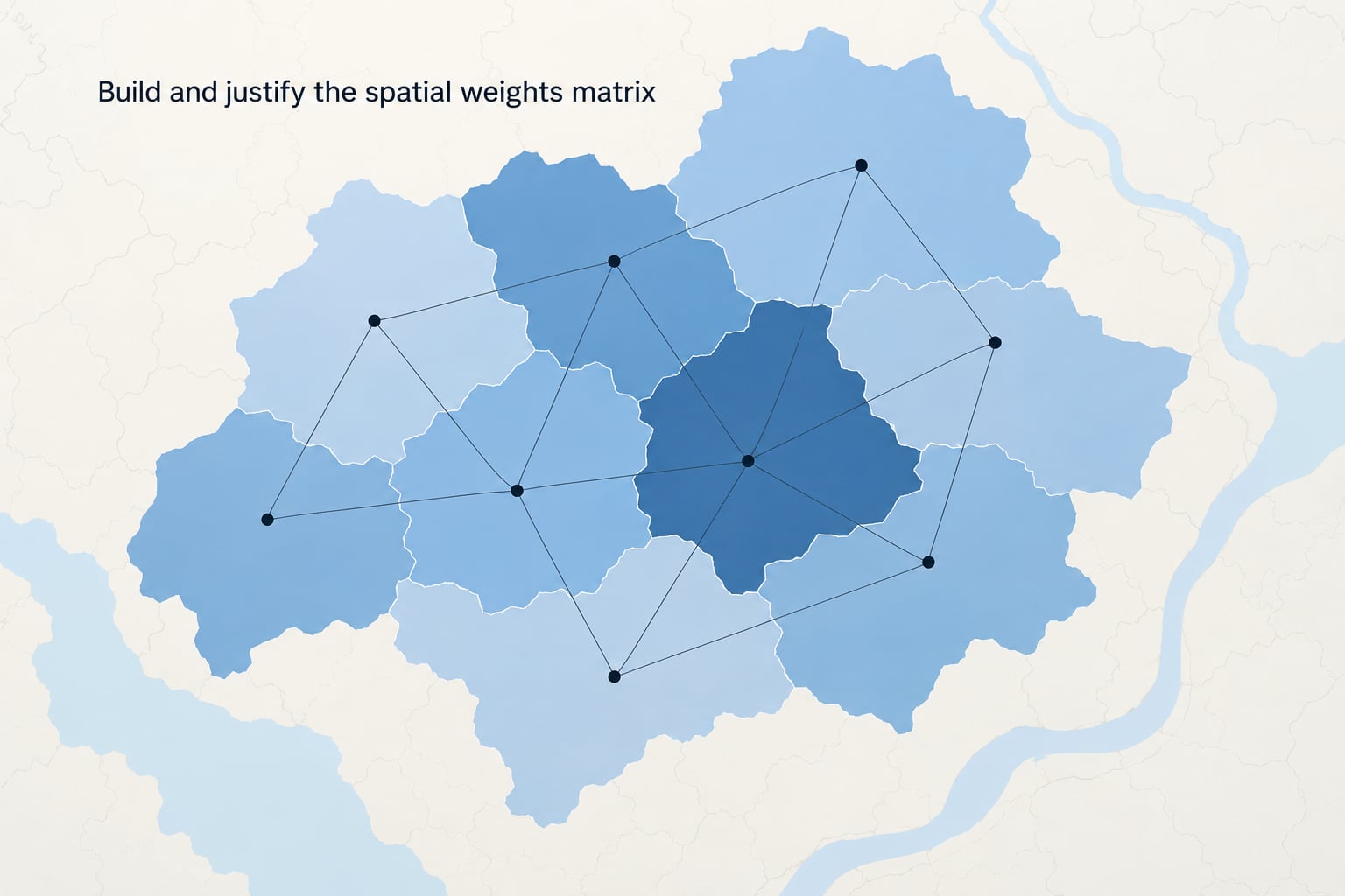
The weights matrix W tells each unit which other units count as its neighbours and how much each one counts. Everything downstream depends on this choice, so it deserves a sentence in your methods section.

Four constructions cover most work:

Rule	How neighbours are defined	Fits when	Effect on the statistic
Queen contiguity	Polygons sharing any edge or corner	Areal units such as counties or districts	Many neighbours, weak dilution, often the highest I
Fixed distance band	Everything within a stated distance	Points, or when a real-world distance threshold exists	Band too narrow isolates units, too wide blurs signal
K nearest neighbours	The k closest units, chosen per observation	Irregular sampling, or a known sampling design	Row totals are always equal, so comparisons across maps hold
Inverse distance	Weight falls off with distance	Process varies continuously over the ground	Near units dominate; sensitive to the power of decay

Next, choose the weighting style. Binary weights are all ones. Row-standardized weights divide each row by its row total, so every unit’s influence sums to one and you are asking “is this unit similar to its own neighbourhood average”. Dormann et al. (2007) recommend row-standardization for almost all analysis, and it is the default in most tools. The style changes the number, so always state which one you used.

First-order neighbours touch. Higher-order neighbours reach two or three steps out, capturing regional spillover, but they also inflate significance if you treat them as if they were local.

Check for islands: units with zero neighbours are dropped or handled separately, and GeoDa, spdep and ArcGIS Pro all flag them. The R function nb2listw() and moran.test() take a zero.policy argument, and setting it to TRUE keeps those observations instead of failing the run. A dataset with many islands is telling you the weights rule is wrong for that data, not that the test is impossible.

Finally, re-run under two or three defensible weight schemes. If the sign flips depending on the neighbour rule, the honest report is that the result is scale-dependent, and you say so.

3. Run Moran’s I in GeoDa

Open GeoDa, start a new project, and add your shapefile or GeoPackage as the dataset. In the toolbar, choose Spatial Weight Matrix, pick the variable that identifies units, and select the conceptualization: contiguity for polygons, k nearest or fixed distance for points. Set the number of neighbours or the distance band, and choose row-standardization. Save the weights file so you can reuse it.

Then open Moran’s I from the same toolbar. Select your analysis field, confirm the weights file, and choose a randomization scheme such as 999 permutations. Run it.

The results window reports the observed Moran index, the expected index, the variance, the z-score, and the p-value, with the permutation count printed at the top. A Moran scatterplot appears in the same view. If your z-score is near zero and the p-value is large, your variable is close to randomly arranged at that grain.

4. Run Global Moran’s I in ArcGIS Pro

ArcGIS Pro uses two geoprocessing tools in sequence. Run Generate Spatial Weights Matrix first. In the Parameters box set Input Features, the Field ID, and the Conceptualization of Spatial Relationships, which mirrors the same four options as GeoDa. Set Number of Nearest Neighbors or Distance Band, and set Row Standardization to ROW.

Then run Spatial Autocorrelation (Global Moran’s I) from the Spatial Statistics folder. Set Input Features, the Field containing the variable, the Weight Matrix File from the previous step, and Randomization to Getis-Ord (1992), which is ArcGIS’s permutation option. Set Number of Permutations to 999. Running it without a weight matrix file is also possible; the tool will build one using whatever conceptualization you set.

The output feature class carries a field with the z-score, and the tool messages panel prints the Moran index, expected index, variance, p-value and permutation count. Menu names have moved slightly between ArcGIS Pro versions, and the Spatial Statistics toolbox replaced the old Spatial Statistics toolbar in Pro, so if you are following an older lab manual, look under Analysis > Tools > Spatial Statistics.

5. Reproduce Moran’s I in R

The spdep workflow is short. This is the sequence:

library(sf)
library(spdep)

nc <- st_read("counties.gpkg")

# project to a projected CRS so distances mean metres
nc <- st_transform(nc, 5070)

# build a neighbour list from shared polygon boundaries
nb <- poly2nb(nc, queen = TRUE)

# row-standardize and list islands so results stay aligned
lw <- nb2listw(nb, style = "W", zero.policy = TRUE)

moran.test(nc$rate, lw, zero.policy = TRUE,
          randomisation = FALSE, nsim = 999)

For point data, swap poly2nb() for knn2nb(knearneigh(coords, k = 4)) or dnearneigh(coords, 0, 0, 50000) for a 50 km band.

The printed output gives you the Moran statistic, the expectation I, an estimate of variance, a z-score against the normal approximation, and a p-value from the permutations. That p-value is what you report, not the z-score.

One habit worth forming: build the neighbour list, then attach row numbers before any subsetting. moran.test() can drop or reuse rows when a unit has no neighbours, and if your variable vector was filtered separately the two get out of step. A quick check is that length(nb) equals nrow(nc).

To run the same analysis in Python, libpysal.weights.Queen.from_dataframe or KNN.from_dataframe builds the weights and esda.Moran(y, w) returns the same estimate, expectation, and simulated p-value. Being able to reproduce a result in a second toolchain is a good way to catch a silent data problem.

6. Interpret the observed Moran’s I correctly

Moran’s I is bounded between -1 and +1 but, with row-standardized weights, is not usually attainable at the extremes. The number that matters is the difference between what you observed and what you would expect by chance, which is E(I) = -1/(n-1).

With 30 units, the expected value is -0.034. With 300 units it is -0.0033. So a value of -0.03 on a small dataset is right at chance, while the same number on a large dataset would be a meaningful negative result. This is the single most misread number in the method, and it is the reason a mildly negative value is not evidence of dispersal.

Observed I relative to E(I) = -1/(n-1)	Pattern	Plain English	Next step
Well above, p below 0.05	Clustered	Similar values sit next to similar values	Map the local clusters, then consider a spatial model
Above, p above 0.05	Weak clustering, not distinguishable from random	A pattern that is not worth reporting	Check the grain, then re-run with another weights rule
At or within a fraction of E(I), p large	Random arrangement	No detectable spatial structure at this scale	Do not generalize this to other scales
Below E(I), p below 0.05	Dispersed	Similar values sit next to different values	Look for checkerboarding or over-regular sampling
Near -1	Strongly alternating	Each unit’s neighbours are its opposite	Rare in real data; check for a coding or lag error

What a significant p-value does not tell you: which units form the pattern, how strong the effect is, or that the structure is meaningful in your study. Moran’s I is a one-number summary, so it cannot locate anything. A large study can produce a significant result on a difference of almost no practical size, and a modest value on a small dataset can be highly significant and equally inconsequential.

Two other reporting details. Report the expected value alongside the observed one, and report the permutation count and randomization method. A bare coefficient is not reproducible.

7. Map the pattern and inspect local results

Global Moran’s I says whether the pattern exists anywhere in the map. It never says where. For that you need a Local Moran cluster map, which runs the statistic for each unit against its own neighbours and assigns one of four categories.

• High-High: a high-value unit surrounded by high-value neighbours. This is a cluster.
• Low-Low: a low-value unit surrounded by low-value neighbours. Also a cluster.
• High-Low: a high-value unit among low-value neighbours. This is an outlier, and often the most interesting category.
• Low-High: a low-value unit among high-value neighbours. Also an outlier.

Not every High-High is a real cluster. Each local statistic comes with its own p-value, and on a map of 200 units you would expect a handful to look extreme by chance alone. Apply a significance threshold such as 0.05 before calling anything a cluster, and say what you used.

Multiple testing is the honest issue here: testing every unit individually inflates false positives, and tools such as GeoDa apply a false discovery rate adjustment to compensate. Use it, and mention it. Disconnected or island units also complicate the local map, since their neighbours may be far away or absent, so a scattered pattern on the map can be an artifact of the weights rather than a real phenomenon.

Finally, a global result near zero can still sit on top of significant local clusters that cancel each other out. The reverse is also true. Always run the local map before writing the interpretation paragraph.

8. Check robustness and report the analysis

Run the test again under at least one alternative weights scheme: a different k, a wider distance band, or queen against rook contiguity. If the sign and rough magnitude hold up, you can say the finding is not an artifact of one neighbour definition. If it does not, say that too, because a reader who re-runs your data will find it anyway.

Diagnose influential units by running the test with and without the extremes, or by examining the scatterplot for points far from the regression line. A single outlier can drive the whole statistic in a small dataset.

Then write it up. A usable reporting template:

Global Moran’s I was computed on [variable] at the [unit] level using [weights construction], row-standardized, with [k] nearest neighbours / a [distance] band. The observed I was [value], compared with an expected value of [value] under a random arrangement. Inference used [n] permutations of the [method] randomization scheme, giving a p-value of [value]. A local Moran cluster map identified [n] significant High-High clusters, [n] Low-Low clusters, and [n] spatial outliers at p below [threshold], using [adjustment]. The result is interpreted as evidence of [clustering / dispersion] in the analysis variable at this spatial scale, not as evidence of a causal process.

Keep that last clause. Spatial autocorrelation describes a pattern, never a mechanism. If you want to say one place influences another, you need a spatial lag or spatial error model, and you need to say so separately.

Common Mistakes

Choosing neighbours arbitrarily. If you cannot write the rule in a sentence, you cannot defend it. Pick a rule tied to the process or to the sampling design, and re-run under one alternative.

Using raw counts instead of rates. A county with more people has a higher count whether or not anything interesting is happening. Use a rate with a stable denominator, and be cautious where denominators are small.

Losing row alignment. Weights matrices are positional. Any subset, merge, or sort of your variable vector after building the neighbour list will misalign it. Check that the identifier column travels with both.

Using distance units that do not match the data. A band of 10 in decimal degrees is not 10 km. Project to a metric CRS first, or state that the band is in degrees deliberately.

Treating the expected value as zero. It is -1/(n-1), not zero. On 20 units it is -0.0526, and a value of -0.04 is closer to chance than most people assume.

Confusing significance with strength. A p-value of 0.001 with an I of 0.05 is weak evidence of a weak pattern. Report the size of I and its distance from the expected value, not just the p-value.

Over-interpreting the global result. It is an average over the whole map. It cannot tell you where the structure sits, and it can hide strong local clusters that cancel.

Using Moran’s I on binary outcomes. Presence-absence and count data violate the normality assumption the statistic leans on. Use Join-count statistics for binary data, or model the outcome directly with spatial-aware methods, and test the model residuals rather than the raw response.

Skipping the parameters. Weights construction, standardization, k or band, permutations, randomization, significance threshold, and any multiple-testing adjustment all belong in the methods paragraph.

Reading a non-significant result as proof of no structure. It is only a statement about this variable, at this grain, with this neighbour rule. Change any one of the three and the answer can change.

Frequently Asked Questions

Conclusion

Start today by checking three things: that your identifier is unique, that your analysis variable is numeric with no nulls, and that you know your spatial grain. Then build a row-standardized weights matrix with a neighbour rule you can defend in one sentence, run Global Moran’s I with 999 permutations, and open a local Moran cluster map before you write a single word of interpretation.

Compare the result to the expected value of -1/(n-1), not to zero, and report the observed I, the expectation, the p-value, the permutations, the randomization method, and the weights construction in the same sentence. If you plan to run a regression on this data, test the residuals, not the raw variable, and expect to follow up with a spatial lag or spatial error model.

That is how to run spatial autocorrelation and interpret Moran’s I without overstating it. This walkthrough was checked against current documentation in October 2026; menu paths in ArcGIS Pro do shift between versions, so confirm the tool names in your own install.