How to Determine Sample Size for Regression Analysis 2026

You determine the sample size for a regression by running an a priori power analysis before you collect any data, entering four quantities: the smallest effect you want to be able to detect, the significance level, the statistical power you need, and the number of predictors in your model. G*Power returns the minimum number of observations that satisfies those four constraints in about thirty seconds. The 10-observations-per-predictor rule gets quoted constantly, and it is fine as a floor, but it is not an answer.

Here is the whole process, including a worked example that produces N = 61 before any attrition allowance, and the code to reproduce it in R.

One warning up front. If you arrived here from a survey-research guide, close that tab. Formulas built on confidence level, margin of error and a z-score estimate a proportion. They do not apply to regression, no matter how confidently a blog states otherwise.

Table of Contents

1. 1What You Need Before You Calculate Sample Size for Regression
2. 2Step-by-Step: How to Determine Sample Size for Regression Analysis
3. 3Step 1: Define the Regression Model
4. 4Step 2: Choose a Target Statistical Power
5. 5Step 3: Set the Significance Level and Minimum Effect
6. 6Step 4: Calculate the Required Sample Size
7. 7Step 5: Adjust for Attrition and Missing Data
8. 8Step 6: Report and Justify the Decision
9. 9Common Mistakes That Ruin a Regression Sample Size
10. 10Frequently Asked Questions
11. 11Is there a minimum number of observations for regression analysis?
12. 12Can I determine regression sample size using the 10-observations-per-predictor rule?
13. 13Which regression sample-size calculator should students use?
14. 14What happens if my regression sample is too small?
15. 15Do categorical variables and interaction terms increase the required sample size?
16. 16Conclusion

What You Need Before You Calculate Sample Size for Regression

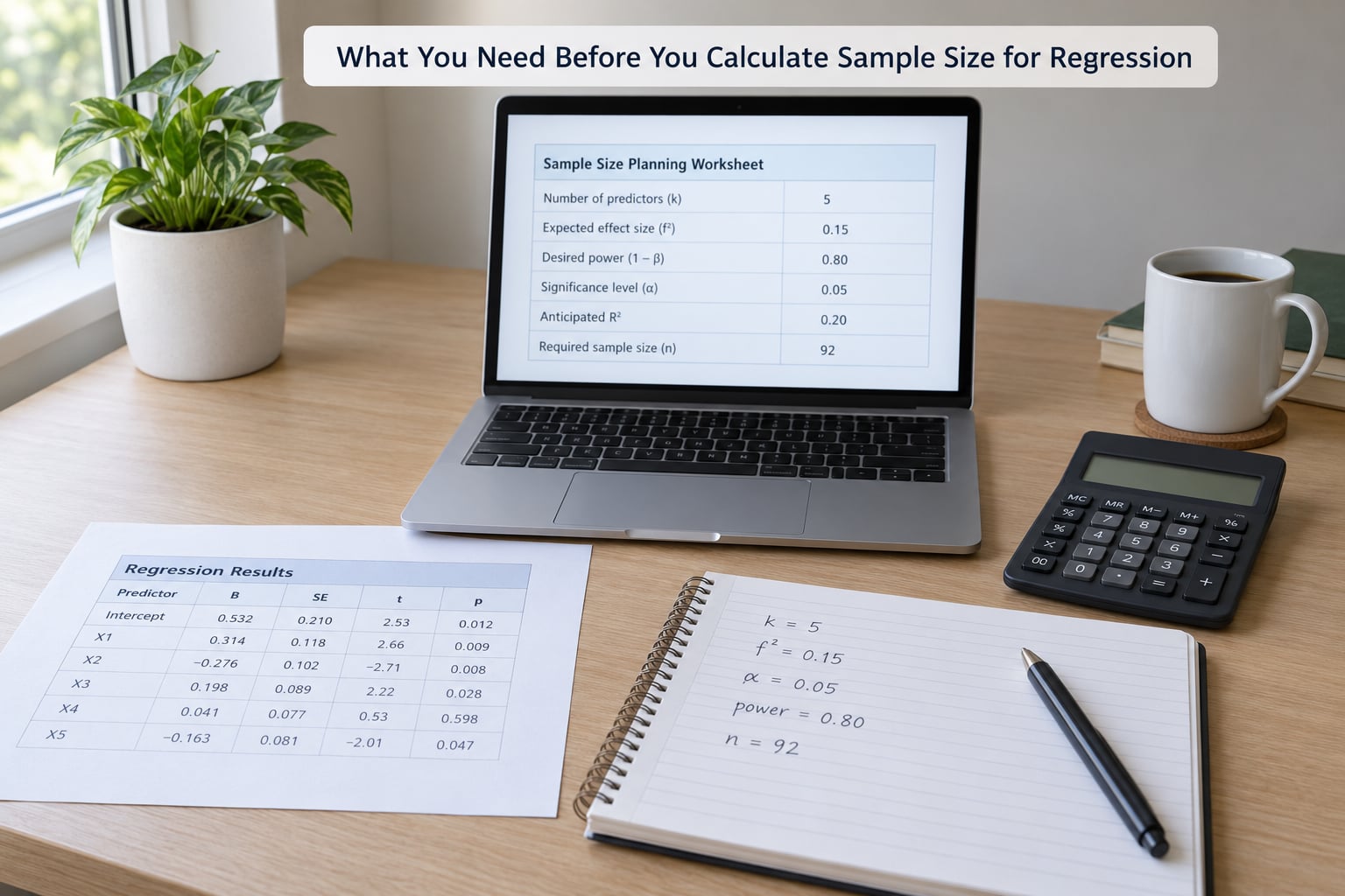
You need seven things lined up before the calculation means anything. Skipping any one of them is how people end up with a number they cannot defend in a proposal.

• Your regression model. The outcome variable, whether it is continuous or binary, and therefore whether you are sizing a linear model or a logistic one.
• The smallest effect worth detecting. Not the effect you hope for. The smallest one you would still care about if it turned out. In linear regression this is usually expressed as an R-squared increase or as Cohen’s f.
• A significance level. Almost always 0.05 for a single primary hypothesis, and something stricter once you adjust for multiple tests.
• A target power. Usually 0.80, which means an 80 percent chance of detecting that minimum effect.
• A correct predictor count. Every continuous predictor is one. A categorical predictor with k levels costs k minus 1. Every interaction adds its own parameters.
• An attrition estimate. The share of recruited cases you expect to lose to incomplete responses, exclusions or unusable records.
• Software. G*Power 3.1, which is free on Windows, macOS and Linux, or the pwr package in R if you prefer to script it. Both give the same answer for the same inputs.

If you can fill in those seven, you are ready. If the effect size is the one you cannot name, read Step 3 next, because that is where most real projects stall.

Step-by-Step: How to Determine Sample Size for Regression Analysis

Step 1: Define the Regression Model

Start by writing the full model equation on paper, predictors on the left and the outcome on the right. The count of parameters in that equation is your numerator degrees of freedom, and it is the single most commonly miscounted input.

A continuous predictor costs one degree of freedom. A categorical predictor with k levels costs k minus 1, because one level becomes the reference group and the model only estimates contrasts against it. So a four-level employment-status variable is three degrees of freedom, not one. An interaction between two predictors is its own predictor, and an interaction between a continuous and a four-level variable costs three.

Decide also what kind of regression you are running. Multiple linear regression for a continuous outcome, logistic regression for a binary outcome, ordinal regression for ordered categories, or something multilevel if your cases are nested. Each has its own test family in the software, and swapping families quietly changes the answer.

Write the count down: it becomes the u or numerator df input in Step 4.

Step 2: Choose a Target Statistical Power

Power is the probability that your test finds the effect when a real effect of that size is there. Set it before you look at N, because it is one of the two levers that determine N.

0.80 is the field default and the right choice for most exploratory and thesis work. If your study is confirmatory, difficult to repeat, or powered by a funding review board, 0.90 buys you a stronger guarantee at the cost of roughly 20 to 30 percent more cases. Going above 0.90 usually buys very little and inflates recruitment badly.

Two things power is not. It is not a probability that your conclusion is correct. And it is not a guarantee of significance: a study with 0.80 power still misses one real effect in five, so plan to interpret a null result cautiously rather than as proof of no relationship.

Step 3: Set the Significance Level and Minimum Effect

Alpha is the long-run rate of false positives you accept, and 0.05 is the default. If you are testing several primary hypotheses, correct before you calculate. Bonferroni simply divides alpha by the number of tests; Holm’s step-down procedure is less conservative and usually the better choice. Powering your analysis at an uncorrected alpha and then correcting at analysis time is planning to be underpowered.

The minimum effect is the hard one. Here is how to pick it honestly.

First choice, prior research in your area. Take a recent study with the same outcome and a comparable predictor, read the partial R-squared for the specific effect you care about, and use something slightly below it. You are planning to detect a bit less than what has already been observed, not exactly what was observed.

Second choice, Cohen’s conventions. They are conventions rather than laws, but they remain a defensible anchor when nothing else is available.

Cohen’s f and the R-squared increase it corresponds to

Effect size	Cohen’s f	R-squared increase	Reading
Small	0.10	0.01	Explains about 1 percent of variance
Medium	0.25	0.06	Explains about 6 percent
Large	0.40	0.14	Explains about 14 percent

The conversion runs in both directions through a simple formula: R-squared increase equals f squared divided by one plus f squared. So if prior work reports a partial R-squared of 0.05, f is roughly 0.23, close to medium.

Third option, and the honest one for a new area. Plan for a small effect, accept that you will need a large N, and say in your methods section that you used a small effect because no prior estimate existed. Reviewers accept that. What they do not accept is a medium effect chosen with no reason attached, which is what most people end up doing.

A fourth option is to run a pilot. Collect 20 to 30 cases, estimate the partial R-squared for your target predictor, and use that value as your planning input, then apply the usual safety margin and treat the pilot’s effect size as provisional. Pilots work best for instrument-heavy studies where measurement error makes the effect size genuinely unknown in advance.

For logistic regression, the effect size input is usually an odds ratio, and the same logic applies. Rough equivalents to Cohen’s small, medium and large are 1.5, 2.0 and 2.65, though prior odds ratios beat benchmarks every time.

Step 4: Calculate the Required Sample Size

This is where the four inputs go in, and the process takes about a minute in G*Power. Open the program and set the dropdowns in this order.

1. Test family: F tests.
2. Statistical test: Linear multiple regression.
3. Type of analysis: A priori. Never post hoc, and the reasons are in the mistakes section below.
4. Type of model: Fixed model, with the correction set to regression coefficients 1.
5. Test: R-squared increase. This is the right choice when the full model adds predictors to a smaller model.
6. Effect size: enter Cohen’s f, 0.25 for a medium effect.
7. Alpha: 0.05, two-tailed. Use one-tailed only if the direction was specified before you saw any data.
8. Power: 0.80.
9. Number of predictors: your count from Step 1, 5 in the example.
10. Click Calculate. Read the sample size from the right-hand column.

That returns N = 61 for five predictors, alpha 0.05, power 0.80 and a medium effect. Try it yourself and confirm you land on the same figure before you build anything on top of it. G*Power also has a sensitivity option in the same dropdown, where you enter the N you already have and it returns the power that N delivers. Run both and compare: the two numbers should sit close together when your inputs were sensible.

If you would rather work in R, the pwr package does the same calculation in one line. Leave v unset and the function solves for the sample size.

library(pwr)

pwr.f2.test(u = 5,          # predictors, from Step 1
            v = NULL,       # NULL = solve for sample size
            f2 = 0.25,      # Cohen's f: 0.10 small, 0.25 medium, 0.40 large
            sig.level = 0.05,
            power = 0.80,
            type = "multiple.regression")

The same script works as a sensitivity sweep, which is what you run when the required N is larger than the population you can reach. Plot power against N across a range and read off the minimum N that clears 0.80.

candidate_n <- 40:200
power_at <- sapply(candidate_n, function(n)
  pwr.f2.test(u = 5, v = n - 6, f2 = 0.25,
              sig.level = 0.05, type = "multiple.regression")$power)

plot(candidate_n, power_at, type = "l", lwd = 2,
     xlab = "Sample size", ylab = "Power")
abline(h = 0.80, lty = 2)
abline(v = min(candidate_n[power_at >= 0.80]), lty = 2)

Knowing where that curve flattens changes the conversation with your supervisor. A study with N = 60 at power 0.79 and a study with N = 60 at power 0.55 are not the same study, and the curve makes the difference visible.

Approximate required sample sizes, alpha 0.05 and power 0.80, fixed model, R-squared increase test:

Approximate N by predictor count and effect size

Predictors	Small (f = 0.10)	Medium (f = 0.25)	Large (f = 0.40)
1	118	34	15
2	130	39	18
3	145	45	22
5	184	61	31
8	261	92	50
10	325	117	65
15	480	176	100

Two patterns jump out. Adding predictors costs far more in the small-effect column than the large one, because a weak model needs precision about each coefficient. And the difference between powering for a small and a medium effect is often the difference between a feasible and an impossible project. Run the small column before you promise anyone a number.

Logistic regression uses the odds-ratio input instead. It also has its own floor, the events-per-variable rule: aim for at least 10 outcome events per estimated parameter, with 15 to 20 preferred when the outcome is rare or the model has interaction terms. Peduzzi and colleagues showed the original 10-events rule fails once you pass roughly 10 parameters.

Logistic regression sizing with 8 parameters and a 20 percent base rate

Target	Events needed	Total N
10 events per parameter	80	400
15 events per parameter	120	600
20 events per parameter	160	800

A rare outcome changes everything. Drop the event rate from 20 percent to 5 percent and the 80 events you needed now require roughly 1,600 cases. Always calculate from events, never from total N alone.

If your accessible population is genuinely small, run the sweep above over the range you can actually achieve and report the power you get. A transparent study with N = 45 at power 0.70 is defensible. A study that quietly claims power 0.80 it never had is not.

Step 5: Adjust for Attrition and Missing Data

The number G*Power gives you is the minimum analyzable sample, not your recruitment target. Divide it by the proportion of usable records you expect.

With N = 61 and 15 percent expected loss, 61 divided by 0.85 gives 72 cases. With 20 percent loss it is 77. Recruitment panels that promise a 30 percent completion rate should be treated as a 30 percent loss, not as a rounding issue.

Inflating a required N of 61 for attrition

Expected loss	Recruitment target
5 percent	65
10 percent	68
15 percent	72
20 percent	77
30 percent	88

Round up to a number you can actually field, then keep it. Also plan for the awkward exclusions that hit after collection: cases with impossible values, straight-lined scale responses, influential outliers. Between 10 and 15 percent is a normal allowance for a self-report survey, and a pilot is the only reliable way to sharpen the figure for your own instrument.

Step 6: Report and Justify the Decision

A sample size justification is one short paragraph in your methods section, and it should contain every input so a reader can reproduce it. State the analysis type, the effect size and where it came from, the alpha level and any adjustment, the power, the predictor count with the degrees of freedom contributed by categorical variables and interactions, the resulting N, the attrition allowance, and the software with its version.

Write it like this: a priori power analysis for a fixed-effects multiple linear regression with five predictors, using a medium effect of f = 0.25 based on prior findings, alpha of 0.05 and power of 0.80, gives a minimum of N = 61; inflating by 15 percent for incomplete responses yields a recruitment target of 72. Analysis was planned in G*Power version 3.1.9.2.

Then add the honest caveats. If you used Cohen’s benchmarks rather than prior research, say so. If your population is capped below the calculated N, say that too, and report the power your achieved sample delivers. Ethics boards and journal reviewers look for exactly these sentences, and their presence usually shortens the review.

Common Mistakes That Ruin a Regression Sample Size

These are the errors that come up again and again in forums and supervisor meetings, roughly in order of how often they happen.

Treating 30 as a universal minimum. The Central Limit Theorem says something about the sampling distribution of a mean, not about regression coefficients. Thirty observations supports a very small number of predictors with very large effects and nothing else. Size the model you have.

Using the survey formulas. Confidence level, margin of error, z-score and the 385 sample figure all estimate a proportion. Feeding a margin of error into a regression design will hand you a number that looks reasonable and means nothing.

Post hoc power analysis. Calculating power after you have seen the results, using the observed effect size from your own data, is circular: a large observed effect always produces high power, and a non-significant result always produces low power, no matter what the truth is. Journals increasingly ask for it anyway; when they do, report the a priori calculation instead, or report the sensitivity sweep from Step 4. The same objection applies to the reverse test, post hoc minimum detectable effect.

Picking a medium effect because the box is there. Cohen’s medium is a placeholder for not knowing. If you power on it and find nothing, you cannot tell whether there is no effect or you looked with a net built for the wrong size. Use prior research, or power for small and accept a larger N.

Counting categorical predictors as one. A four-level variable costs three degrees of freedom. Undercounting here silently produces a sample that is too small for the model you actually specified.

Ignoring what interactions cost. Each interaction adds parameters and pushes the required N up sharply. A moderation study with one interaction routinely needs two to three times the sample of the same main-effects model. Calculate the moderation model, not the main-effects model.

Adjusting alpha after powering. If you plan five primary hypotheses, power the design at alpha divided by five, or use Holm and power at a slightly stricter alpha. Correcting afterwards costs you power you did not buy.

Forgetting attrition. Recruiting the exact minimum means finishing underpowered. Inflate first.

Confusing stable coefficients with detectable significance. These are different targets, which is why G*Power sometimes returns fewer cases than 10 per predictor. Power analysis asks how large N must be to detect an effect; the rule of thumb asks how large N must be for coefficient estimates to settle. When reviewers want reliable estimates rather than a significance test, an accuracy-in-parameter-estimation approach such as Kelly and Maxwell’s is the better frame.

For reference, the shortcuts themselves:

Rule-of-thumb formulas, their sources and their limits

Approach	Rule	Source	Limitation
Ten per predictor	N = 10q	Common practice, no formal derivation	Untested at q above about five
Fifteen to twenty per predictor	N = 15q to 20q	Practitioner guidance for stable coefficients	Costs recruitment fast
Green	N = 5 + 5q	Green (1991)	Optimises for coefficient stability, not power
Barcikowski	N greater than 5 + 5q	Barcikowski and colleagues (1990)	Valid over a wider q range than the ten-per-variable rule
A priori power analysis	Software output	Cohen (1988)	Requires an honest effect size
AIPE	Confidence width target	Kelly and Maxwell (2003)	Answers a different question than significance

Use the rules of thumb as a sanity check on your powered result. If G*Power says 61 and 10 per predictor says 50, both are fine and you have learned nothing alarming. If G*Power says 40 and the rule of thumb says 90, power an extra scenario or two before committing.

Frequently Asked Questions

Conclusion

Write the model down first, then count its degrees of freedom properly. Pick the smallest effect you would still care about, set alpha at 0.05 and power at 0.80, run the a priori analysis in G*Power, and inflate the result for attrition before you commit to a recruitment figure.

That single afternoon of planning is what separates a study that can answer its question from one that collects a pile of data and hopes.