How to Combine Spatial and Statistical Analysis in One Study (2026)

To combine spatial and statistical analysis in one study, you prepare the spatial layer and the statistical table separately, put both onto the same coordinate reference system and the same geographic unit, join one to the other, then run ordinary statistical tests alongside location-aware tests such as spatial autocorrelation and spatial regression. The map shows you where the pattern sits; the statistics tell you whether it would show up again by chance. Treat them as two halves of one argument, not two separate projects.

This is where most student and early-career projects go wrong. Someone maps a variable, someone else runs a regression in a different spreadsheet, and the two halves sit in different chapters with no shared unit of analysis. Fixing that is mostly a matter of deciding the unit and the question first, then letting the data follow. A full workflow takes a few days of careful preparation and an afternoon of actual analysis.

Table of Contents

1. 1What You Need
2. 2Pick a research question that is genuinely spatial
3. 3Understand the three spatial data types
4. 4Have the statistical data in a clean table
5. 5Choose software that covers both halves
6. 6Decide the spatial scale in advance
7. 7Set up a reproducible project folder
8. 8Step-by-Step: How to Combine Spatial and Statistical Analysis in One Study
9. 9Step 1: Define a Research Question That Combines Space and Statistics
10. 10Step 2: Choose the Spatial and Statistical Data You Need
11. 11Step 3: Prepare and Clean the Spatial Data
12. 12Step 4: Explore Spatial Patterns Before Testing Inferences
13. 13Step 5: Run the Statistical Analysis at the Correct Spatial Scale
14. 14Step 6: Test Whether Location Matters
15. 15Step 7: Combine the Spatial and Statistical Results
16. 16Step 8: Report the Combined Study Reproducibly
17. 17Common Mistakes
18. 18Mixing coordinate reference systems
19. 19Ignoring spatial dependence
20. 20Reading a map as proof of cause
21. 21Falling into the ecological fallacy
22. 22Ignoring the modifiable areal unit problem
23. 23Double counting in a spatial join
24. 24Comparing counts across different geometry types
25. 25Letting the boundary version change mid-project
26. 26Frequently Asked Questions
27. 27What is spatial statistical analysis?
28. 28What are the three types of spatial data?
29. 29What is the difference between spatial analysis and spatial statistics?
30. 30What software combines GIS and statistics?
31. 31Do I need a spatial regression if my data is mapped?
32. 32How do I check for spatial autocorrelation?
33. 33Conclusion: Start With the Research Question and Unit of Analysis

What You Need

You need six things before you write a line of code: a research question that genuinely has a geographic component, a defined unit of analysis, at least one spatial layer, at least one statistical table covering the same places and the same period, software that can do both jobs, and a plan for saving the work so someone else can repeat it.

Pick a research question that is genuinely spatial

A question is spatial when removing location would make it meaningless. Is asthma concentrated near a road corridor? Which neighbourhoods have the highest rate relative to their population? That is spatial. Do more people in bigger cities live near transit? That is mostly a count question until you add distance or a rate.

Students on research forums like r/ArcGIS report this exact struggle, asking how to frame a feasible seminar question that needs both kinds of analysis. The test that works: write the question, then underline every word that refers to a place. If nothing is underlined, add a geographic comparison or you have a statistics project, not a combined one.

Understand the three spatial data types

Point, line and polygon are the three types of spatial data you will meet, and each one supports different analysis. A raster cell is a fourth format that behaves differently again.

Type	Geometry	Typical example	Supports
Point	A single coordinate	Clinic locations, tree surveys	Point pattern analysis, kernel density, network accessibility
Line	A connected path	Roads, rivers, cycle routes	Network analysis, buffer analysis, length and density measures
Polygon	An enclosed area	Census tracts, wards, parcels	Choropleth mapping, areal interpolation, spatial regression on zones
Raster	A grid of cells	Elevation, land cover, satellite imagery	Kriging, surface modelling, zonal statistics

Most combined projects end up on polygons, because that is what administrative statistics are published against. Points and lines still matter: Eurostat’s work merging statistical and geospatial data for Poland converted point and line layers into density per square kilometre before comparing them with area-based indicators. Raw counts over different feature types are not comparable.

Have the statistical data in a clean table

One row per geographic unit, one column per variable, an identifier that matches the spatial layer exactly. That is the whole requirement. Bring the table in as a CSV if you can, and keep the identifier column as text so codes with leading zeros survive the trip.

Choose software that covers both halves

You need a geographic information system layer that can handle geometry and a statistics environment that can handle inference. Most stacks let one package do both, which is why the choice comes down to language preference and project size rather than capability.

Stack	Strongest for	Key packages or tools	Watch out for
R	Statistical modelling, spatial regression, reproducible reports	sf, spdep, gstat, lm	Steeper setup than desktop GIS
Python	Scalability, large data, integration with general analysis	geopandas, libpysal, esda, scikit-gstat, rasterio	More assembly required per step
ArcGIS Pro	Point-and-click exploration, hot spot and cluster tools	Spatial Statistics toolbox	Command line scripting takes longer
QGIS	Mapping and data preparation for free	Processing toolbox, joins by location	Spatial statistics are limited

R gets the edge when the work is statistical, because its modelling functions work out of the box on data frames, while Python wins on very large datasets and machine learning pipelines. A 2026 head-to-head comparison of the two for geospatial work makes that same call. Many analysts end up using R for the model and QGIS for the map, exporting a CSV in between, and that handoff is perfectly defensible as long as you document it.

Decide the spatial scale in advance

The geographic unit is the atom of your study: the ward, the grid square, the county, the catchment area. Everything else follows from it. Statistics published for one boundary set will not drop onto another without interpolation, and choosing a different boundary set later can change your findings. Fix the scale before you start downloading files.

Set up a reproducible project folder

Open a project folder now with data, scripts, figures and output inside it, and put raw data in data/raw with every downloaded copy read-only. Write cleaning steps as a script rather than clicking through a desktop interface, because the moment you need to rerun after one late data correction, manual steps become the reason the project stalls.

Step-by-Step: How to Combine Spatial and Statistical Analysis in One Study

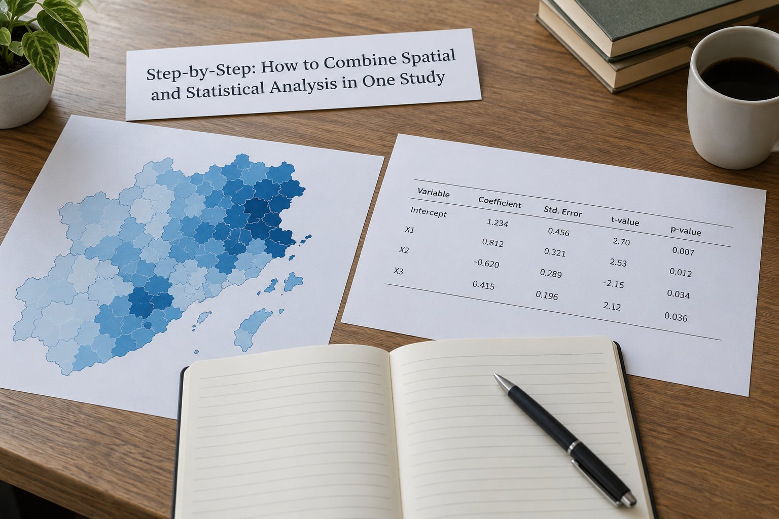
The workflow below takes one research question from a blank page to a reported result, keeping the statistical and spatial halves tied to the same geographic unit throughout. Eight steps, and the two that catch out most beginners are step three and step six.

Step 1: Define a Research Question That Combines Space and Statistics

Write a question with six filled-in slots: the study area, the unit of analysis, the outcome variable, the explanatory variables, the spatial pattern you expect, and the population you are comparing against.

“Are asthma rates in London higher in neighbourhoods within 500 metres of a major road than elsewhere, after adjusting for deprivation and population density?” fills all six. The expected pattern is a gradient near roads; the comparison population is non-adjacent neighbourhoods in the same city. Compare it with a vaguer version, “air pollution and health in London”, which fills none and will drift for months.

Checking your question worked: someone else could run it without asking what outcome, which variable, or which area. If your question mentions a rate, an exposure, a distance, a cluster, a hot spot, an accessibility measure, a boundary or a density, it has a spatial component you can test.

Step 2: Choose the Spatial and Statistical Data You Need

Identify datasets where each layer has a clear job: boundaries define your units, the outcome table supplies the numbers, contextual layers supply the explanatory variables. Then check that dates and geographic coverage actually overlap, which is where published statistics most often disappoint.

Do this check with real numbers. Take three zones from your study area and look up each one in the statistical table by hand. If two of three fail to match, you have an identifier or boundary mismatch and you will find out now rather than after the regression. Record the vintage of every dataset on a single sheet, because pairing an exposure layer from one period with an outcome table from a later one is a limitation a reviewer will flag.

Know the difference between vector data, which stores shapes, and raster data, which stores values in cells. Points, lines and polygons are vector. A land cover or elevation surface is raster. Most combined projects mix them, which means you need a rule for extracting raster values onto polygons before any statistics run.

Step 3: Prepare and Clean the Spatial Data

Project every layer to one coordinate reference system before touching it, then run the quality checks. Geographic coordinates in degrees will give you nonsense distances and areas; a projected system in metres or feet gives you measurements you can defend.

The specific tasks: drop records with missing or obviously wrong coordinates, remove duplicate geometries, fix invalid or self-intersecting polygons, and confirm that every boundary identifier has a match in the statistical table. Then check the join direction and the count of matched rows before you continue.

import geopandas as gpd
zones = gpd.read_file("data/raw/zones.gpkg").to_crs(epsg=27700)
stats = gpd.read_file("data/raw/zone_stats.csv", dtype={"zone_id": str})
merged = zones.merge(stats, on="zone_id", how="left", validate="one_to_one")
print(len(zones), len(stats), merged["outcome"].isna().sum())

The final line prints the three numbers that matter: rows in the spatial layer, rows in the table, and matched rows missing an outcome. Zero missing means the key matched cleanly. A number above zero means your identifiers disagree and you have to trace it before proceeding. Using validate="one_to_one" turns duplicate keys into an error instead of a silently inflated table.

The same attribute join in R is short:

library(sf)
library(dplyr)
zones <- st_read("data/raw/zones.gpkg")
stats <- read.csv("data/raw/zone_stats.csv", stringsAsFactors = FALSE)
merged <- left_join(st_as_sf(zones), stats, by = "zone_id")

There are two different joins here and they are not interchangeable. An attribute join adds columns because identifiers match. A spatial join adds attributes because shapes overlap or lie inside one another. A third option, areal interpolation, redistributes known values from one set of zones onto another by area weighting, and it is the honest answer when your statistics and your boundaries genuinely do not line up.

Before you leave this step, convert counts to rates where the comparison matters. A ward with 300 cases and 2,000 residents is not a bigger problem than one with 60 cases and 400 residents. Divide by population and multiply by a constant, and state the constant in the caption.

Step 4: Explore Spatial Patterns Before Testing Inferences

Map the variable before you model it. Summary statistics hide everything interesting about geography, and the map tells you which problems to expect: a cluster, a gradient, a clear outlier, or an oddly shaped area that is really a data error.

Run four checks together: a histogram or distribution plot of the raw variable, a choropleth map using a classed or quantile scheme, a scatterplot of the outcome against each explanatory variable, and a check of whether any map class is driven by one enormous zone. If your map is one dark polygon against a field of light ones, look at that polygon before you interpret the pattern.

You are done with this step when you can state in a sentence what the spatial pattern appears to be. That sentence becomes the motivation for the formal test in step six.

Step 5: Run the Statistical Analysis at the Correct Spatial Scale

Match the statistical unit to the design. With one observation per person and no clustering, a t-test or a logistic regression is right and location is context. With one observation per neighbourhood, observations sit inside a city and inside a borough, so your model needs to account for grouping.

Two situations cause the most trouble. First, when your individual data sit inside geographic clusters, use a multilevel model with the cluster as a grouping level, because a plain regression treats 4,000 people in one postcode as 4,000 independent facts when they are not. Second, when you aggregate individual data up to zones before modelling, you have changed the question and changed your uncertainty, so say so.

Working at the wrong scale produces confident, wrong answers, which is why this step comes before the spatial tests.

Step 6: Test Whether Location Matters

Location matters when nearby observations resemble each other more than distant ones. That dependence is spatial autocorrelation, and ordinary statistical tests assume it is absent, which is almost never true for geographic data.

Test for it with a global statistic such as Moran’s I, which compares the value at each zone to the average of its neighbours through a spatial weights matrix that defines who counts as a neighbour. A positive and significant value indicates clustering; a negative value indicates alternation, where high zones sit next to low ones; a value near zero suggests a random layout.

import esda, libpysal
from libpysal.weights import Queen
w = Queen.from_dataframe(merged, use_index=True)
moran = esda.Moran(merged["outcome"], w)
print(round(moran.I, 3), round(moran.p_sim, 4))

A significant Moran’s I is the finding that tells you ordinary least squares is not enough here, because the standard errors are too small. The fix is a spatial lag model, which adds a weighted average of neighbouring outcomes to the right-hand side, or a spatial error model, which puts the dependence in the error term instead. Choose the lag when your theory says that a neighbour’s outcome affects this one, such as peer effects or contagion; choose the error when you suspect unmeasured spatially structured factors.

Run a local Moran’s I as well, because the global statistic averages away the local structure. Local results, sometimes called a LISA cluster map, label each zone as high-high, low-low, high-low or low-high and let you see which specific places drive the global clustering. The Getis-Ord statistic answers the related hot spot and cold spot question for counts and rates.

You have handled location correctly when you can state the global result, name the specific areas driving it, and either explain why your model does or does not include spatial terms.

Step 7: Combine the Spatial and Statistical Results

Now write the argument that ties the two halves together. Start from the model, report coefficients with confidence intervals and test values, then point to the map and say which places those coefficients describe. A significant coefficient on road distance plus a map showing elevated rates along the same corridors is a coherent finding. Two maps with no numbers is an illustration.

Watch the interpretation step, because this is where combined studies usually overreach. A map showing clustering does not prove that proximity causes the outcome. It is consistent with shared causes that vary by place, and your confidence interval tells you how precisely you estimated the relationship, not whether the direction of causation is correct.

If you have both individual and aggregate data, check the direction they point before you commit. Findings that hold at both levels are stronger than findings at one, and a disagreement between levels is itself a finding worth a paragraph rather than a footnote.

Step 8: Report the Combined Study Reproducibly

Report in this order: study area and unit of analysis, data sources with vintages, any transformations including projection and rate conversion, the statistical model with its specification, the spatial diagnostic results, then results as table plus map plus prose. Put maps and tables in the same results section, because the point of combining them is that they are read together.

Give every map a caption that names the variable, the unit, the class scheme and the source. State the software and package versions, because spatial weights choices differ between releases. List the diagnostics you ran, including the ones that came back negative, and name your limitations in plain terms: scale sensitivity, coverage gaps, and the ecological inference problem described below.

Before submitting, run the pre-flight check: does every figure regenerate from a clean run of the scripts, does every table number match its source object, does every map have a stated class scheme, and can a reader tell which dataset produced each column.

Common Mistakes

These are the errors that recur in combined spatial and statistical work, with the fix for each. Most of them come from treating the map as decoration rather than as part of the inference.

Mixing coordinate reference systems

Two layers in different projections will either fail to join or join to the wrong neighbour, and in the worst case produce plausible-looking but wrong distances and areas. Project everything to one CRS before the first operation and record which one you picked in the methods section.

Ignoring spatial dependence

Running ordinary regression on clustered data gives standard errors that are too small, which means p-values you report as significant are less certain than they look. Test for autocorrelation first, and move to a spatial model when the test comes back significant. Mapping the data is not a substitute for this test.

Reading a map as proof of cause

A visible cluster is a hypothesis, not a mechanism. A shared unmeasured factor, such as deprivation or housing quality, can produce the same picture. Support a causal claim with a design that addresses confounding, and describe the rest as association.

Falling into the ecological fallacy

Properties of zones are not properties of the people in them. A ward with high average income tells you nothing certain about any household there. This matters most when you only have aggregate data, which is the normal case for administrative statistics. State the limit plainly and avoid wording like “residents in these areas are”.

Ignoring the modifiable areal unit problem

Both the scale and the zoning of your units change your results. Redissolve your zones into larger ones, or shift to a regular grid, and check whether your key findings survive. If they flip, that is a limitation to report, not a detail to leave out.

Double counting in a spatial join

Joining points to overlapping polygons matches each point to every polygon it falls in, so one clinic can count twice or three times. This is the single most common complaint on geospatial forum threads about joining tables to polygon layers. Dissolve overlapping polygons first, match points to one zone each, or write the join to keep only the smallest containing polygon.

Comparing counts across different geometry types

A business count and a road length are not comparable numbers, and neither is comparable to a population count across zones of different size. Convert both to densities, such as businesses per square kilometre, before you compare or map them. Keep the conversion constant consistent and state it.

Letting the boundary version change mid-project

Boundary files get revised, and a mismatched version silently changes which zone a record belongs to. Pin one boundary release, store it in your project, and record its identifier and date.

Frequently Asked Questions

Conclusion: Start With the Research Question and Unit of Analysis

A combined spatial and statistical study is one study with two outputs, not two studies stapled together. The workflow runs from a precise research question, through a fixed unit of analysis, clean and projected spatial data, a verified join, exploratory mapping, a correctly scaled statistical model, a spatial dependence test, and finally a results section where maps and tables are read together.

Your first action is small and concrete. Write the question with the six slots filled in, name the geographic unit, open your statistical table and your boundary file side by side, and check whether three sample zones match on both. If they do, the rest of the workflow follows from that decision. If they do not, you have found your real blocker, and you can fix it in an afternoon rather than after writing a chapter of analysis.